In Situ Hyperspectral Remote Sensing for Monitoring of Alpine Trampled and Recultivated Species


1
Department of Geoinformatics, Cartography and Remote Sensing, Faculty of Geography and Regional Studies, University of Warsaw, 00–927 Warsaw, Poland
2
Pixalytics Ltd., Plymouth PL6 8BX, UK
*
Author to whom correspondence should be addressed.
Remote Sens. 2019, 11(11), 1296; https://doi.org/10.3390/rs11111296
Submission received: 15 March 2019
/
Revised: 2 May 2019
/
Accepted: 23 May 2019
/
Published: 30 May 2019
(This article belongs to the Special Issue OPTIMISE: Innovative Optical Tools for Proximal Sensing of Ecophysiological Processes)
Abstract
:Vegetation, through its condition, reflects the properties of the environment. Heterogeneous alpine ecosystems play a critical role in global monitoring systems, but due to low accessibility, cloudy conditions, and short vegetation periods, standard monitoring methods cannot be applied comprehensively. Hyperspectral tools offer a variety of methods based on narrow-band data, but before extrapolation to an airborne or satellite scale, they must be verified using plant biometrical variables. This study aims to assess the condition of alpine sward dominant species (Agrostis rupestris, Festuca picta, and Luzula alpino-pilosa) of the UNESCO Man&Biosphere Tatra National Park (TPN) where the high mountain grasslands are strongly influenced by tourists. Data were analyzed for trampled, reference, and recultivated polygons. The field-obtained hyperspectral properties were verified using ground measured photosynthetically active radiation, chlorophyll content, fluorescence, and evapotranspiration. Statistically significant changes in terms of cellular structures, chlorophyll, and water content in the canopy were detected. Lower values for the remote sensing indices were observed for trampled plants (about 10–15%). Species in recultivated areas were characterized by a similar, or sometimes improved, spectral properties than the reference polygons; confirmed by fluorescence measurements (Fv/Fm). Overall, the fluorescence analysis and remote sensing tools confirmed the suitability of such methods for monitoring species in remote mountain areas, and the general condition of these grasslands was determined as good.
1. Introduction
During evolution, vegetation has developed alternative metabolism paths and defense reactions that enable it to grow in unfavorable conditions, as well as regenerate damage, which is referred to as resistance to stress, disturbance, and competition [1,2]. One of the crucial factors causing stress in vegetation is trampling [3,4], including crushing and defragmentation of organs [5]. Adaptation of plants to difficult conditions is observable in their leaf construction, leaf resilience as well as stem flexibility and extended root system. This impacts the so-called tolerance to the trampling of a particular species [6,7]. Due to extensive environmental changes, in most cases, the passive protection of nature does not guarantee that the extinction of a species or ecosystem degradation will stop [8]. Therefore, it is necessary to explore the measurement of plant parameters and properties in order to assess ecosystem functioning [9,10], especially in valuable natural and hard-to-reach high-mountain ecosystems.
Hyperspectral remote sensing involves analyzing numerous narrow bands of electromagnetic radiation that enables the repeated monitoring of vegetation in a quantitative and qualitative manner, but must be verified by biometric measurements such as chlorophyll content or chlorophyll fluorescence [11,12]. In fact, researchers refer to the measurement of fluorescence as the barcode of physiological properties of a specific plant, which may be used e.g., for taxonomic purposes [13]. Fluorescence is the quantity of absorbed light (quanta) leading to excitation of chlorophyll particles that have not been used in photosynthesis due to stressors [14]; both abiotic and biotic. Therefore, the measurement of chlorophyll fluorescence is believed to be the best photosynthesis efficiency index [15] for most species, i.e., not exposed to stressors. Optimal fluorescence (Fv/Fm) rates are approximately 0.83 with adaptation to darkness [16,17]. High photosynthetically active light intensity is characteristic of alpine plants, causing stress [18], similarly, a decrease in the air temperature to −2°C brings about a reduction of the Fv/Fm ratio [19]. Even though alpine vegetation reduces the negative effects of strong sunlight exposure [20] by numerous adaptations, still, a combination of several stressors (e.g., dryness) will result in browning of leaves, lower biomass production, poorer photosynthesis productivity [21,22] and a loss of turgidity [23]; simultaneously, one may observe lower Fv/Fm rates (stress index).
In order to better explain the mechanism functioning in high-mountainous plants, and their true state of health, biophysical measurements and biometric values are commonly used for verifying spectral information. This can be through assessing the so-called APAR (Absorbed Photosynthetically Active Radiation) and fAPAR (fraction of Absorbed Photosynthetically Active Radiation) rates, moreover, a measurement of thermodynamic air temperature (ta) and plant canopy radiation temperature (ts), can assess water stress through a temperature ts-ta index rate and Chlorophyll Content Index (CCI). In addition, modern methods often use remote sensing indicators to model biometric values. For example, regression models have been used to perform quantitative analyses between spectral VIs and LAI [24] or CCC (Canopy chlorophyll content) [25] measured under different phenological stages. In such analysis models, such as PROSPECT and SAIL radiative transfer models (PROSAIL) [26], multiple linear regression (SMLR; [27]), partial least square regression (PLSR; [28]) or multivariate adaptive regression splines (MARS; [29]) are often used. In addition, the coefficient of determination (R2) and RMSE are employed to evaluate the outputs. An advantage is these non-invasive methods can be shifted from ground-based to airborne [30] or satellite monitoring [11,12], e.g., the ESA FLEX satellite mission [31].
Research published about vegetation within the Tatra National Park has gradually evolved. Initially, the difference in trampled and reference vegetation was tested using only a ground-based spectrometer [32] with spectral curves and remote sensing vegetation indices analyzed. In subsequent years, for the purpose of their verification, chlorophyll (CCI) and accumulated energy (fAPAR) measurements in the area of Kasprowy Peak and the surrounding area were added to broaden the scope to verification [33]. Next, in order to check the methodology, the research was transferred to another TPN area—the Red Peaks, where the obtained test results were verified, and the methods were extended by applying chlorophyll fluorescence measurements to check what actual damage occurs during plant trampling [34].
Assessing vegetation trampling has developed over several years [32,33,34,35] focusing on new verification methods as well as the application of research by park employees. The current paper presents an analysis based on field studies, with an emphasis on recultivated areas; not previously measured. The goals are an assessment of spectral ranges and remote sensing indices, which were carried out by dividing the swards into trampled and reference polygons. However, along with the development of tourism in the Park area, protective measures were applied to the most degraded areas that are also a focus of this article.
This study tested the hypothesis that there is potential for using various hyperspectral vegetation indices for estimating, modeling chlorophyll fluorescence and chlorophyll for different types of alpine swards species. A key aspect of the research was finding the appropriate parts of the electromagnetic spectrum that can be used for ground, airborne and satellite level monitoring of plants. Another aspect was the correlation between remote sensing indices, plant physiology metrics (chlorophyll content and its fluorescence), absorption of accumulated energy for photosynthesis (APAR) and evapotranspiration. The precise determination of indicators and ranges of the spectrum for species will allow for the analysis of the condition and monitoring of individual protected species in the National Park.
2. Study Area and Research Objects
The Tatra Mountains are the highest mountain range between the Alps and the Caucasus. The Tatra National Park (Tatrzański Park Narodowy, TPN) covers 21,197 ha of the Polish part of Tatras, out of which 11,500 ha are under strict protection (all high-mountain ecosystems). The whole area of the Tatra Mountains includes two national parks: the TPN and the Tatranský Národný Park (TANAP), which jointly created the UNESCO Man & Biosphere nature reserve and met the criteria of the Special Protection Area (OSO) and Special Conservation Area (SOO). It is marked by a characteristic alpine landscape with a typical Central European climate with strong influences from Oceanic and Continental climates modified by altitude. Plant zones containing abundant flora (about 1000 species of vascular plants) and fauna include many species that are rare or endangered in Poland [36]. Owing to the multitude of habitats and species, the area of the Tatra Mountains has been qualified as a Natura 2000 area. Alpine swards are exposed to high insolation and overheating and, simultaneously, strong and cold winds can cause considerable water loss. Thus, local vegetation has developed a range of protection mechanisms, such as succulent leaves and leaves covered with tomentum and wax. Due to the high altitude above sea level, the plants are smaller and less common. Their short height can protect them from unfavorable exposure to cold winds, with the whole plant able to survive under the snow. Alternatively, they may grow again from underground parts in the case of a shortened vegetation period [37]. Also, some alpine plants have green leaves with a high chlorophyll content, which ensures rapid vegetation and blooming, allowing them to set fruit after the snow is gone.
The research area included the vicinity of the Kasprowy Peak, Beskid, Gąsienicowa Valley and Red Peaks (Kopa Kondracka, Ciemniak, Figure 1), with the focus being vegetation growing in selected fragments of the alpine and subalpine floor termed alpine swards. Based on a list of precious flora kept by the Polish Chief Inspectorate for Environmental Protection, as well as maps of real vegetation [38], dominant alpine sward species, i.e., Agrostis rupestris, Festuca picta and Luzula alpino-pilosa, were selected and subject to an in-depth analysis. These species grow on the most precious mountain areas where, from April to September, about 75% of the annual tourist traffic is concentrated. The observed phenomenon of strong anthropopressure leads to intense exploitation of the land, resulting in destruction and restructuring of the plant cover and soil erosion in the areas neighboring trails [39,40].
Agrostis rupestris is a narrow-leaved grass growing in tufts with 5–20 cm long raised blades [41]. Its leaf blades are rolled, whereas the corymb may reach a length of 4 cm; the plant blooms in July and August and grows both on swards as well as on mountain pastures, having a typically scree-type nature [42]. What is characteristic of the plant is its resistance to trampling, e.g., [37,43]. Mirek and Piękoś-Mirek [44] described Agrostis rupestris as a native species that has adapted to anthropogenic habitats. Festuca picta belongs to the Poaceae family and grows in thick tufts [37,45]. Its leaf blades are curved and filamentous, with a width of up to 0.7 cm, with the sole distinctive feature being the red-brown-violet color of inflorescences, which consist of numerous two-to-three-millimeter spikelets. Festuca picta has very low habitat requirements. Luzula alpino-pilosa, which belongs to the family of Juncaceae, grows as dense fields on snow patch communities in humid couloirs, on gravels, screes, rocks, and banks of streams. This green plant, with leaves of approx. 2–7 mm width, will grow up to a height of 30 cm [44] and blooms at the end of July and August. Its inflorescence is scattered and branched, whereas the flowers are inconspicuous and small. They grow on stalks, 2–3 on each, and have a dark brown, almost black, color [44].
3. Materials and Methods
The measurements commenced by selecting the research polygons, including vegetation monitoring networks operated by the TPN and Polish Railways (Polskie Linie Kolejowe). All the polygons were broken down to: (a) areas subject to trampling, which are located in the neighborhood of trails, at sites clearly destroyed by tourists; (b) reference areas with similar habitat conditions located near to trampled areas but normally at a distance of 10 m from trampled polygons; (c) recultivation areas, i.e., patches delineated by the TPN with limited access; where the species are planted under biodegradable jute mats that help them to grow and make it easier for them to attach to the ground. For all the areas, homogenous tufts of individual species were identified; all the measurements were conducted on species to eliminate the potential influence of other species, rocks and soils on the spectral properties. The polygon locations were recorded using a GPS Trimble GeoXT to an accuracy of 50–70 cm so that the same polygons could be analyzed in later years.
For each polygon, all species were examined (the trampled, reference and recultivation patches: Agrostis rupestris—98 polygons, Luzula alpino-pilosa—77 polygons, Festuca picta—28 polygons). Ten sets of measurement were undertaken for each polygon each year, in accordance with the following order (Figure 2):
- Identification of individual tufts of homogenous species through taking documentary photographs;
- Spectral properties using an ASD FieldSpec 3 (ASD Inc., Longmont, CO, USA) spectrometer using a fiber optic cable at an angle of 25° from a plant’s surface at a distance of about 1 m2 [32], as well as the ASD PlantProbe (ASD Inc., Longmont, CO, USA) in order to keep identical measurement conditions in all years [32]. Prior to each series of measurements, the spectrometer was calibrated using a white Spectralon tile (SG 33151 Zenith Lite Reflectance Target and calibration screen P/N A122634 Leaf clip). Thanks to the application of a probe, it was possible to precisely register the properties of individual species, eliminating the influence of the environment on the spectral reflectance curve. In total, 4115 × 25 spectrometric measurements were performed with the sets of 25 independent measurements automatically averaged and recorded as one out of 4115 measurements;
- Leaf chlorophyll content measurements using a Chlorophyll Content Meter CCM-200 (OptiScience, Inc. Opti-Sciences, Inc., Hudson, NH, USA) that measures the Chlorophyll Content Index (CCI).
- Chlorophyll fluorescence using the Plant Stress Meter fluorometer (PSM Mark II, Biomonitor, Stockholm, Sweden) and LeafClip applied to create a dark adaptation that terminates the photosynthesis processes. Measurements were also performed without dark adaptation. As the first stage, a measurement of leaves without adaptation to darkness (i.e., the Fv’/Fm’ fluorescence rate), then a second stage measurement with adaptation to darkness (a leaf fragment was put in the dark using a LeafClip, the Fv/Fm fluorescence rate); then, after about 30 min of being in the dark, a final measurement was performed that allowed all the chlorophyll pigments to be excited by a light impulse.
- Air thermodynamic temperature (ta) and leaf radiation temperature (ts) using the IRtec MiniRay 100 with an insert probe pyrometer (Eurotron Instruments S.p.A., Milan, Italy) in order to evaluate the water stress using the thermal infrared (TIR). Measurements were conducted in accordance with the 30:1 parity, which means that if the distance to the plant amounted to 30 units, the diameter from which information was gathered equaled to 1 unit. In practice, when measuring a single plant species, the measurement was performed at a distance of about 3 m from a studied tuft, with a circle whose diameter was about 10 cm that was equivalent to the canopy of a given species.
- Measuring energy balance of Absorbed Photosynthetically Active Radiation (APAR) and the fraction of APAR (fAPAR = APAR/PARo) [25] by measuring its components (PAR0—total radiation incoming to the canopy, PARc—canopy reflected PAR, PARt—PAR transmitted through the canopy, PARs—soil-reflected PAR) using a line ceptometer AccuPAR model 80 (Decagon Devices, Pullman, Washington, USA) [46].
3.1. Calculation of Remote Sensing Vegetation Indices
The spectra gathered during the ASD FieldSpec 3 spectrometric studies were exported to an ASCII format and then converted using the Statistica 13 software. As a result, one could calculate remote sensing vegetation indices in individual study periods and for individual patches, as well as compare the spectral reflectance curves. Based on previous experience [32,33], the number of indices was narrowed down so as to focus on those showing a statistically significant difference (Table 1) and to check their usefulness in the case of recultivated species.
3.2. Statistical Analysis of Data
Statistical analyses were conducted using the Statistica 13 software (TIBCO Software Inc., Palo Alto, CA, USA) [61]. Each of the species examined in the research period 2012–2014 was analyzed separately. The analysis of spectral reflectance curves based on the Ward’s method of data agglomeration enabled a comparison of spectra characteristics of alpine sward species. It allowed an observation of which species have similar spectral characteristics in all three cases of polygons (trampled, reference and recultivated, respectively) and which species are most like one another in the reflectance 350–2500 nm range. For all the analyses, the level of statistical significance amounted to α = 0.05 and involved the following steps:
- Analysis of variance (ANOVA) The ANOVA analysis showed which ranges of the electromagnetic spectrum are statistically differentiated between polygons (trampled, referenced and recultivated) for each tested species and sites.
- The difference in remote sensing vegetation index values between the tested polygons for each of the three species was also checked. The procedure of statistical indicator analysis had the following structure:
- The ANOVA Kruskal-Wallis one-way analysis of variance by ranks was applied (due to the lack of normal data distribution) to analyze the species differences for each situation (trampled, reference and recultivated). This information was acquired through multiple comparisons (so-called post hoc comparisons)—in the present case, the Tukey’s HSD test was selected.
- The correlation of calculated remote sensing indices is based on spectral reflectance curves and biophysical variables. Because the distribution of both type of indicators: calculated from the spectral reflectance curve and biometric indicators (defining biophysical variables), was not normal then Spearman’s rank-order correlation coefficient was applied (Rs).
- Multivariate adaptive regression splines (MARS) were used to forecast the object condition based on remote sensing indices and biophysical variables (selected in the course of the prior statistical analysis) that showed a statistically significant relationship with the alpine sward species. Based on all the measurements conducted, a model for the Fv/Fm (n = 1600 cases) and CCI (n = 2400 cases) rates were created for the dominant alpine sward species (excluding the verification area, which in this case was the Red Peaks). The occurrence of interactions means that the influence of an independent variable (X1) on a dependent variable (Y) is different, depending on the level of the next independent variable (X2) or a series of successive independent variables. One may speak of an interaction or combination of two factors when the reaction of a studied feature at the level of one factor is not the same on all levels of the other factor [64]. A model was developed per parameter as well as the Generalized Cross Validation error (GCV), which demonstrates an error in cross-validation, i.e., proves whether a model matches real data. Moreover, the GCV parameter accounts for both the residual error and the extent of model complexity. In order to implement the research methodology for remote monitoring of alpine sward condition, e.g., hyperspectral imaging, the researchers attempted to verify the model in the Red Peaks area. And so, the rates modeled based on spectrometric data were compared with the rates determined in the field, using independent bioradiometric measurements, and then presented in the form of the coefficient of determination (R2), whereby the closer the rates to one, the more the model matches real data.
4. Results
Spectrometric measurements conducted in the field confirmed spectral differentiation of species within the study area; the differences were statistically significant for species growing in trampled and recultivated areas compared to those in the reference areas. The condition of the vegetation in the aforementioned areas was different, and the plants located next to trails with heavy tourist traffic were mainly characterized by a poorer state. Whereas the vegetation from recultivated areas was characterized with similar conditions as the species in reference polygons.
4.1. Differentiation of Spectral Characteristics
Spectral characteristics of studied species differed among one another depending on the condition of the vegetation and the species. Spectral differences were confirmed between trampled plants (_T), recultivated (_Rec) and reference plants (_R). Depicting spectral characteristics using the Ward’s method demonstrated a degree of similarity for spectral reflectance rates in individual species. The greatest influence exerted by trampling on spectral properties occurred in the polygons and differentiation of the spectral characteristics in three tested polygons was also observed for Luzula alpino-pilosa (LAP_T, LAP_R, LAP_Rec) and in sequence Agrostis rupestris (AR_T, AR_R, AR_Rec). The most similar research polygons from these three species tested (reference and trampled in terms of spectral properties for one species) were found to be the ones containing Festuca picta (FP_T, FP_R). This does not mean that this species did not show any difference between trampled and reference areas; however, this difference in spectral characteristics was less clear than the two previous species. This means that in the hierarchy of resistance to trampling, we can consider this species as resistant, in relation to the other two. Similar spectral characteristics were concluded in the reference polygons for the species Luzula alpino-pilosa and Agrostis rupestris (LAP_R, AR_R), and also the spectral characteristics of these species are similar to each other in the trampled polygons (LAP_T, AR_T; Figure 3).
Comparing the spectral characteristics of dominant alpine sward species allowed the researchers to identify spectrum ranges, demonstrating statistically significant differences and showing changes in spectral properties that depended on the plant species trampled, recultivated or reference. What all the species under research had in common, were ranges demonstrating absorption of photosynthetically active pigments, water content in the canopy, content of dry matter and building substances such as proteins and nitrogen (Table 2).
The reflected, statistically significant, range of electromagnetic radiation is different for each studied species, demonstrating narrower/wider ranges. Grayed out statistically significant ranges of the spectrum determine the highest probability (95%) of occurrence of differences in the spectral characteristics between all polygons for the studied species (Figure 4). This dependence results from adaptations of a given plant as well as its leaf structure, which reflects changes in a given species brought about by trampling. The spectral characteristics of Agrostis rupestris demonstrate a better cell structure condition in remediated plants compared to reference plants; in addition, one may observe a lower reflectance coefficient rate in the range demonstrating water content in reference plants. This means that water content is higher in those polygons as water absorbs electromagnetic radiation (Figure 4).
Visible destruction of trampled vegetation could be observed through a lower absorption in the red range; this is a sign of a lower chlorophyll level in the plant, e.g., Festuca picta. A flattened red edge and lower reflectance in that range were observed, depicting cell structure as well as higher reflectance values in the range describing water content pointing to its lower level (Figure 4). Moreover, recultivated vegetation is characterized by considerably higher, statistically significant, change in the water content and number of pigments; especially of chlorophyll, e.g., Luzula alpino-pilosa.
Summing up, it should be noted that spectral characteristics of the dominant alpine sward species demonstrate the condition of the vegetation, which may be deemed good in the case of reference and recultivated vegetation (as no changes in the red edge range were detected). Flattening is observable only in the case of trampled plants, whose cell structures are subject to destruction. The impact of trampling is visible in the chlorophyll and cell structure (in particular—red edge) as well as the content of building material. Trampled vegetation also shows lower water content (a statistically significant range from 1801–2500 nm). Hence, the condition of trampled plants is poorer due to lower absorption in the red electromagnetic spectrum as compared to the reflectance in the green range, which points to a lower chlorophyll content.
4.2. Utility of Remote Sensing Vegetation Indices
The calculated remote sensing vegetation indices and biometrical variables (CCI, ts-ta, fAPAR, Fv’/Fm’, Fv/Fm) also show statistically significant changes for the three species of high-mountain grassland between the types of the polygons. Specific groups of vegetation indices showing high correlation with the biometrical variables indicating water and biomass content in the canopy, plant pigment and general condition of vegetation between trampled and reference polygons (Table 3). In the case of recultivated polygons, the Spearman rank correlation coefficient (Rs) was below 0.50, which is why it was not included in the table below. The table shows the correlation coefficient Rs above 0.50 and only statistically significant cases (at 0.05 statistically significant level). The indicators that show the highest number of occurrences in correlation with biophysical variables include (in order from the most numerous ones): WBI—Water Band Index, CAI—Cellulose Absorption Index, NDWI—Normalized Difference Water Index, PSRI—Plant Senescence Reflectance Index, ARVI—Atmospherically Resistant Vegetation Index, PRI—Photochemical Reflectance Index, NMDI—Normalized Multi-band Drought Index, RARSa—Ratio analysis of reflectance spectra algorithm chlorophyll a, SIPI—Structure Insensitive Pigment Index, NDNI—Normalized Difference Nitrogen Index (Table 3).
For the monitoring of reference and trampled species, the most useful are indices presenting canopy water content, e.g., WBI (Figure 5). Species in trampled areas showed a drop of 0.1 to 0.4 in WBI compared to the reference and recultivated areas (Figure 5). The lowest WBI was observed in the case of Luzula alpino-pilosa growing in trampled areas (LAP_T), while the highest water content was determined for Luzula alpino-pilosa (LAP_R) growing in reference areas, as well as Agrostis rupestris from recultivated areas (AR_Rec). Luzula alpino-pilosa may serve as an example, as the statistically significant difference between the reference and the trampled areas for this species amounts to 0.05, which also confirms the results for the Ward method for this species, which proved to be sensitive to trampling.
The above remarks were confirmed by the ts-ta temperature index, which in some cases pointed to water stress (positive values, >0 of the ts−ta temperature index) and weakened evapotranspiration capacities. The species that demonstrated water deficit included: Agrostis rupestris and Festuca picta in trampled areas (AR_T, FP_T). The water stress indicator for the remaining species was within the thresholds of a general median for this indicator, with a value of −3.50°C, i.e., fell within the optimum range.
The next group of statistically significant indicators in the study of high-mountain vegetation describe dry or senescent carbon. The cellulose content reflected by CAI in the dominant species of alpine swards is variable and depends on the structure of a given species. Higher values point to greater cellulose content was observed for alpine swards growing in trampled areas. The highest CAI values were determined for Festuca picta, while in each of the measurement periods Luzula alpino-pilosa grew in trampled, reference and recultivated areas that demonstrated the lowest cellulose content (Figure 6). This is not always related only to the process of trampling, but also to the construction and specificity of the species. This information is also confirmed by PSRI, where the common range for green vegetation is −0.1 to 0.2. This index maximizes the sensitivity of the index to the ratio of bulk carotenoids (for example, alpha-carotene and beta-carotene) to chlorophyll. An increase in PSRI indicates increased canopy stress (carotenoid pigment), the onset of canopy senescence, and plant fruit ripening e.g., AR_T, LAP_T and FP_T (Figure 6).
The general condition of plants can be monitored based on the absorption of photosynthetic active radiation measured by the ARVI. In the case of the ARVI index, higher values indicate a better condition, which was detected for: Agrostis rupestris, Luzula alpino-pilosa and Festuca picta growing in reference and recultivated areas (Figure 7). Also, changes between the trampled and reference areas were observed, with the greatest changes detected for Luzula alpino-pilosa and Agrostis rupestris (0.16; Figure 7).
The highest productivity in alpine sward species, growing in areas subject to recultivation, was observed by indicators from the group described light use efficiency. As far as alpine swards are concerned, PRI rates from −0.14 to 0.04 with higher rates demonstrating a better use of light in the photosynthesis process, implying better productivity and a lack of damage in the plant cells; in turn, a drop in the rate suggests worst functioning vegetation. The median PRI rates for all studied species (in the case of reference and recultivated areas) are higher than the respective rates in trampled plants, which have a general median of below 0.035 (Figure 8). This means that alpine sward vegetation growing in trampled areas is exposed to additional stress that weakens it.
The productivity data have also been verified using fAPAR. For alpine swards in recultivated and reference areas, this indicator reached median values of approx. 0.9 in particular species, which suggests high utilization of light for photosynthesis (Figure 8). In contrast, in species growing in trampled area, this rate was reduced; also, a considerable interquartile gap (which is the range between the upper and lower quartile) was observed in 50% of the cases. An increased fAPAR rate suggests better plant productivity; looking at plants from reference areas a significant correlation with ARVI (Rs = 0.74) and RARSa (Rs = −0.72) was observed for Luzula alpino-pilosa; this plant has intensely live-green leaves.
Measurements of chlorophyll content (CCI) and chlorophyll fluorescence (Fv/Fm; Fv’/Fm’) can be used as a confirmation of good condition. The highest CCI index correlation was with the ARVI (Rs = 0.80) as well as the PRI (Rs = 0.78) for Festuca picta, which points to the good development of vegetation (Figure 9), and this confirmed the earlier observed resistance to trampling compared to the other two species. Yet, in the case of trampled polygons the strength of correlation was either negative or very low. For instance, in the case of Luzula alpino-pilosa CCI showed a statistically significant correlation with CAI (Rs = 0.73), reflecting a drop in the cellulose content in trampled vegetation (Table 3).
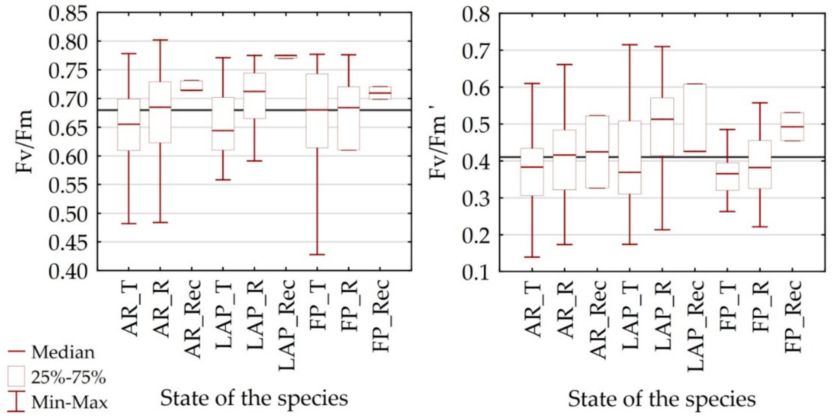
Information on the fluorescence processes derived from remote sensing vegetation indices was confirmed by fluorescence (both with and without adaptation to darkness) and is presented as the form of a correlation (Table 3). Alpine sward species growing in reference areas showed a high correlation between Fv/Fm and PRI, e.g., in Festuca picta (Rs = 0.65). The values of Fv/Fm’ showed the greatest strength of correlation with PRI (Rs = 0.60—for Festuca picta from reference polygons); CAI (Rs = 0.51 Agrostis rupestris from trampled patches). The fluorescence measurements verified the actual condition of the photosynthetic apparatus. The median rates for Fv/Fm (adaptation to darkness) range from 0.650 to 0.810 for species in reference areas (Figure 10). When subject to trampling, they are significantly lower and below 0.700. For all the species, the median Fv/Fm measured was 0.653 while Fv’/Fm’ (without adaptation) was 0.398. Fluorescence measurements also confirmed the gradation of resistance to trampling (from the most to least resistant species): Festuca picta, Agrostis rupestris, Luzula alpino-pilosa.
4.3. Estimation of the Chlorophyll Content Basing on Spectral Properties of Dominant Alpine Species
A wide set of hyperspectral indices (ARVI, NMDI, RARSa, GI, SIPI, NDNI, PSRI, CAI, WBI, NDWI) and the multivariate adaptive regression splines method (MARS) modeled the chlorophyll (CCI) and its fluorescence (Fv/Fm) indices. The accuracy of modeling was confirmed by GCV (Generalized Cross Validation error), R2 and RMSE rates (Table 4). The RMSE error determined for the Fv/Fm model ranged from 12 to 20%, whereas for the CCI model it accounted for 11 to 16%. Both Fv/Fm and CCI point to a relatively robust model adjustment of the forecasted index; hence they may be applied for the purpose of forecasting the actual condition of fluorescence and chlorophyll content in the studied alpine sward species.
5. Discussion
Species differences for areas located next to tourist trails, experiencing trampling, were expected. The largest percentage of change (80–100%), for species across the whole electromagnetic spectrum, was for Luzula alpino-pilosa and Agrostis rupestris. In the case of Luzula alpino-pilosa, it was related to the wide structure of the leaf blade as well as its thickness and size; implied considerable destruction from trampling. The leaves and stems of Festuca picta are harder, so trampling led to a smaller percentage of change (50–60%), which was also true for Agrostis rupestris. Similar conclusions were presented by Balcerkiewicz [65], who reasoned that grazing caused the plants to grow in succession, with grassy vegetation transitioning to intermediate communities between grassy plants, alpine swards and matgrass swards.
Oprządek [66] also observed that the closer to the trail, the more common species, e.g., Agrostis rupestris, which builds single-species patches along paths; negative and statistically significant correlations were achieved for three quantitative categories (total number of occurrences, quantity above 1 and >3). The strongest correlation (Rs = 0.902), was recorded for the last category (>3, i.e., above 50%), which indicated the dominance of this species along the trail and may indicate its greater resistance to trampling. This was confirmed by the observations of Mirek and Piękoś-Mirek [44], who defined Agrostis as a native species that has adapted to anthropogenic habitats and often becomes dominant. Its presence next to tourist trails was also noted by Górski [67], who described the community of Agrostis rupestris occurring on tourist paths and in other trampled places.
Remote sensing measurements made it possible to broadly categorize the state of the plants in terms of the effect of trampling. Based on the vegetation indices and biometrical variables, the resistance to trampling (from most to least resistant species) was: Festuca picta, Agrostis rupestris and then Luzula alpino-pilosa.In the studies conducted by Oprządek [66], Luzula alpino-pilosa demonstrated a poor negative correlation (Rs = 0.382) to the distance from the trail. However, in contrast to Agrostis rupestris, it does not create a hull community and instead finds favorable conditions through habitat (longer snow cover and the formation of gravels or screes on the edge of the path) that means it tends to form monogenous patches along the paths; confirmed by the observations of Mirek and Piękoś-Mirek [44]. Another species that Oprządek [66] referred to as negatively correlated (Rs = 0.793) with the distance from the trail within TPN, was Festuca picta. This confirms our results and the validity of the methods used to monitor changes. The botanical studies conducted so far have not been sufficient, as they only quantify the percentage share of the species in the study area along the trail. Using remote sensing methods, especially chlorophyll analysis and chlorophyll fluorescence, a decrease in condition (by about 10–15%) in relation to reference polygons was determined for plants within trampled polygons.
Table 5 lists statistically significant ranges within the electromagnetic spectrum, which emphasize the differences between the spectral characteristics of the species studied in the three types of research polygons (trampled, reference, recultivated). This can be used to indicate significant wavelengths, with a list prepared on the basis of the wavelengths used within remote sensing vegetation indices, which have proved to be the most useful in showing differences and variability linked to species state. In this study, the greatest differences in species spectral characteristics were for the spectral ranges describing the absorption of photosynthetically active pigments (448–514, 531–707 nm), cell structures (1385–1556 nm), and water content (1801–1835, 1845–1862, 1879–2500 nm; Table 5). These differences also result from specific adaptations to excessive radiation (change in the carotenoid and chlorophyll ratio).
In addition, these spectral ranges have previously been used to assess changes in the vegetation condition by authors such as Ruban et al. [68], Gitelson and Merzlyak [69] or Fourty and Baret [79]. The bands used most frequently to analyze water content, and water stress included 950–970, 1150–1260, 1520–1540 nm [81,82]. The width of ranges (Table 5) relevant for examining alpine swards condition points to the fact that swards may be monitored using satellite sensors as well as airborne hyperspectral imaging. For instance, WorldView-2 and 3 whose channels 2 (450–510 nm) and 5 (630–690 nm) overlap with the ranges deemed significant. Also, WorldView-4 has channels in the blue (450–510 nm) and red (655–690 nm), and similarly RapidEye (blue: 440–510 nm; red 630–685 nm), to which such environmental analyses may be applied.
In this study, the median PRI rates for all species studied (in the case of reference and recultivated areas) are higher than the respective rates in trampled plants, with the latter ranging below the general median of 0.035. This means that alpine sward vegetation growing in trampled areas is exposed to additional stress that weakens it. In the literature, PRI values gradually increased from winter, through spring to summer [83]. Species in trampled areas also showed a drop of 0.1 to 0.4 in WBI compared to reference and recultivated areas respectively. The species that demonstrated water deficiency included: Agrostis rupestris and Luzula alpino-pilosa in trampled areas (AR_T, LAP_T). Changes observable in the vegetation were confirmed by previous research where, due to trampling, significant differences in remote sensing vegetation indices (α = 0,001) for NDWI, NDII and WBI related to water content; ARVI related to general condition; PSRI and CAI related to the quantity of carbon in the dry cellulose matter and lignin as well as PRI related to the amount of light used in photosynthesis [32]. Having determined the change in condition over two years, conclusions were drawn about the influence of weather conditions on vegetation’s state.
Fluorescence demonstrated a poorer condition for plants in trampled areas compared to those growing in reference or recultivated areas. For non-stressed plant material, the Fv/Fm value is expected to be 0.81–0.83 for leaf material dark-adapted for a minimum of 20 min [84]. For reference and recultivated plants, the median rates measured for Fv/Fm fell within the range of 0.700–0.755. When subject to trampling, the measured values were significantly lower and below 0.700 with the median for all species being 0.653 while Fv’/Fm’ (without adaptation) was 0.398. In the literature, values lower by more or less than 0.100 were observed for Fv’/Fm’ compared to Fv/Fm [85]. Therefore, the measurements confirmed the dependence, namely that plants exposed to abiotic and biotic stress show lower than 0.830 or 0.832 ± 0.004 Fv/Fm values [86,87], with a decrease of Fv/Fm and mechanic damage to plant tissues causing disturbed transport within the plant and a drop in biomass and overall robustness [88]. However, high photosynthetically active light intensity can also lead to stress in plants, with a drop in the rate of Fv/Fm [89]. Therefore, in shady sites, trampling can lead to less vegetation damage and a smaller drop in biodiversity [90]. The resulting rates are reduced compared to the optimum Fv/Fm, amounting to 0.780–0.865 [91] or 0.780–0.840 [16]. Overall, measurement of chlorophyll fluorescence allows researchers to detect stress prior to the appearance of visible external symptoms, including poorer growth [92], withering, necrosis and chlorosis [93].
A high correlation coefficient of Fv/Fm with the indices describing the use of light for photosynthesis allows for long-term monitoring of vegetation. In this study, the Fv/Fm index demonstrated a high correlation with indices measuring chlorophyll content and the use of light for photosynthesis e.g., the species of alpine swards growing in reference areas were marked by a high correlation between Fv/Fm and PRI: Festuca picta (Rs = 0.65). The rates of Fv’/Fm’ demonstrated the highest correlation with PRI (Rs = 0.40 for Festuca picta from trampled areas; Rs = 0.60 for Festuca picta in reference areas); and CAI (Rs = 0.51 Agrostis rupestris from trampled areas). Studies which may serve as an example include those conducted by Tan et al. [94], in which the SIPI index strongly correlated with Fv/Fm (R = 0.88) and was used to measure the variability of condition of and damage to maize. Studies of the reaction of maize to volatile levels of hydration were demonstrated by a high correlation between the Photochemical Reflectance Index 570 (PRI570) and Fv/Fm’ (R2 = 0.76); this index turned out to be linked to water stress at an early stage, prior to the occurrence of structural changes in the plant [95]. PRI was most often correlated with actual photochemical efficiency ΔFv/Fm’ and explained 17–90% of its variability; median R2 was higher for conifers (0.50) than for other species groups (Broadleaf 0.40, Herbaceous and crop 0.48 [83]. PRI explained 44–74% of the variability of the actual quantum yield for broadleaved and herbaceous/crop plants but accounted for only 1–40% of the variability of ΔFv/Fm’ for mixed forests [83]. Panigada et al. [96] reported that PRI570 and PRI586 correlated with ΔF/Fm′ (R2 = 0.49 and 0.51, respectively) for cereal crops under water stress better than other PRIs [96]. Compared with PRI, the reflectance ratio R686/R630 also yielded a slightly higher average R2 when related to Chl-Fs and Fv/Fm parameters. The daily R2 values for PRI and R686/R630 was varied between 0.27–0.78 and 0.20–0.70, respectively, such a high variation might be related to the high heterogeneity of leaf angle distribution [97]. This justifies the interpretation of data gathered about the vegetation spectral properties, e.g., the use of light for photosynthesis (PRI) or WBI, being the indicator reflecting water content. PRI was significantly correlated with Fv/Fm, RWC (relative water content), mean R2 between 0.58 and 0.86 [83,98]. The research literature indicates that most stressors affecting the photosynthesis apparatus may reduce the Fv/Fm ratio; some authors confirmed its constant rate during drought conditions [99,100].
By applying the MARS method to this study, the following prediction rates were established: R2 from 0.71–0.96 and RMSE from 2–8% for Fv/Fm, with the R2 falling to 0.68–0.93 and RMSE to 4–7% for CCI. During verification of the Red Peaks model, the following rates were detected: respectively, R2 from 0.58–0.72 RMSE from 12–19% for Fv/Fm, and R2 from 0.54 to 0.75 and RMSE from 11–16% for CCI. Nawar et al. [29] modelled soil salinity and arrived at similar average model accuracies for MARS – R2 = 0.73, RMSE = 6.53 or for content of clay and organic matter was (R2 = 0.81, RMSE = 7.7; R2 = 0.89, RMSE = 6.9; R2 = 0.73, RMSE = 0.34; [101].
6. Conclusions
The present study confirmed the usability of hyperspectral remote sensing for evaluating the condition of vegetation, with the dominant species of alpine swards characterized by a set of unique properties that can be measured using hyperspectral sensors and fluorescence measurements. The most significant properties included plant pigments (and their relative quantity), protective elements such as the leaf shape and structure or leaf cover (especially the wax cover). In addition, this paper represents an interdisciplinary approach, including both remote sensing (by spectrometric and bioradiometric measurements as well as the option of transmitting information to a different level) with ecophysiology (features of leaves) and ecology (management of protected areas); the methods in question combine spectral characteristics and vegetation indices providing data on fluorescence and, hence, allowing a detailed analysis. Hyperspectral measurements, in turn, were used to confirm statistically significant differences in the spectral characteristics of trampled, reference and recultivated vegetation. These observations were confirmed by the chlorophyll content, fluorescence and the ts-ta index; the Fv/Fm fluorescence ratio was used to evaluate chlorophyll condition and the process of photosynthesis. Studies, such as the one presented in this paper, may be repeated temporally to monitor the condition over time; each vegetation season is characterized by varied weather conditions that affect the development of vegetation. Also, the remaining natural and anthropogenic factors vary, which can be captured through monitoring conducted using remote sensing methods. Estimation of the condition of vegetation on recultivated polygons is important from the point of reasonableness the protection of plant cover used by employees of the Park; good condition of vegetation in these areas confirms the validity of recultivated methods of degraded areas.
Summing up, the condition of reference species was good, but the trampled vegetation had undergone visible changes. For this reason, based on statistically relevant changes in all the studied indices, a distribution of species was developed, starting from those that showed the lowest sensitivity to the trampling stressor to those that presented the greatest variability and sensitivity Festuca picta, Agrostis rupestris and then Luzula alpino-pilosa. This demonstrated the usability of hyperspectral remote sensing to evaluate the condition of alpine sward species growing on protected high-mountain areas. The application of non-invasive field measurements allowed for detailed in situ examinations of individual species, especially endemic flora, which is particularly valuable. The rates of spectral reflectance in vegetation growing in reference and recultivated areas were similar, which implies that recultivation is appropriate. The species under analysis reacted in various ways to trampling; this is due to their different structure and adaptations to difficult environmental conditions. As far as trampled plants are concerned, there was a drop in the amount of chlorophyll and water content, as well as a poorer condition of cell structures and decreased photosynthetic productivity.
Spectral width (full width at half maximum, FWHM) is significant when studying the condition of alpine sward vegetation; swards may be successfully monitored using hyperspectral airborne imaging, as well as satellite imaging. Examples of such satellites are WorldView-2 and WorldView-3, where channels 2 and 5 provide between 450–510 nm and 630–690 nm, are deemed significant in this study. Also, WorldView-4, featuring multi-spectral blue (450–510 nm) and red (655–690 nm) channels or RapidEye (blue: 440–510 nm; red 630–685 nm) may be used. However, one should bear in mind the role of the data’s spatial resolution and the impact of soil reflectance, especially in the case of pixels located near trails where the vegetation cover is not complete.
Author Contributions
Conceptualization, M.K., B.Z. and S.L.; Data curation, M.K. and B.Z.; Formal analysis, M.K.; Funding acquisition, B.Z.; Investigation, M.K., B.Z. and A.D.; Methodology, M.K., B.Z., S.L. and A.D.; Project administration, B.Z.; Resources, B.Z. and S.L.; Supervision, B.Z.; Validation, M.K.; Visualization, M.K.; Writing—original draft, M.K., B.Z., S.L. and A.D.; Writing—review & editing, M.K., B.Z., S.L. and A.D.
Funding
The publishing costs were financed from the theme No. 500-D119-12-1190000 awarded by the Polish Ministry of Science and Higher Education.
Acknowledgments
Authors would like to thank the Tatra National Park, Institute of Geography and Spatial Organisation of Polish Academy of Sciences and the Anna Pasek Foundation, which in 2012/2013 funded a scholarship to Marlena Kycko.
Conflicts of Interest
The authors declare no conflict of interest.
Appendix A

| Formula of the Indicator | Accuracy |
|---|---|
| Fv/Fm Agrostis rupestris = 0.627 + 1.92 × max(0; NDNI–0.171) + 1.93 × max(0; 0.171–NDNI) – 34.7 × max(0; CAI+1.93 × 10⁻³) + 8.14 × max(0; CAI+1.69 × 10⁻²) + 1.64 × max(0; RARSa –0.583) + 0.285 × max(0; 0.39–ARVI) – 0.137 × max(0; 2.12–G) + 6.74 × max(0; PRI+3.60 × 10⁻³) + 1.48 × max(0; PSRI–8.79 × 10⁻²) – 4.88 × max(0; 8.79 × 10⁻²-PSRI) – 1.41 × max(0; RARSa–0.493) – 0.266 × max(0; G – 2.48) + 1.57 × max(0; 1.21–SIPI) + 2.31 × max(0; NDWI–4.83 × 10⁻²) | Error GCV = 0.0020 |
| R2 = 0.71 | |
| RMSE = 8% | |
| Fv/Fm Luzula alpino-pilosa = 0.942 + 2.52 × max(0; SIPI – 1.02) + 4.45 × max(0; 1.02–SIPI) + 1.90 × max(0; NDNI–0.197) – 4.37 × max(0; 0.197–NDNI) – 4.12 × max(0; RARSa–0.567) – 4.20 × max(0; WBI–0.936) + 5.88 × max(0; 0.936–WBI) + 3.79 × max(0; NMDI– 0.549) – 0.919 × max(0; 0.549–NMDI) – 0.416 × max(0; 1.94–G) - 5.55 × max(0; ARVI – 0.436) + 2.03 × max(0; ARVI – 0.406) + 3.54 × max(0; ARVI – 0.461) + 1.67 × max(0; NDWI + 1.64 × 10⁻³) – 1.44 × max(0; ARVI–0.527) | Error GCV = 0.0014 |
| R2 = 0.83 | |
| RMSE = 6% | |
| Fv/Fm Festuca Picta = 0.512 + 0.845 × max(0; ARVI – 0.435) – 0.256 × max(0; 0.435–ARVI) – 5.64 × max(0; SIPI–1.07) + 2.74 × max(0; 1.07–SIPI) + 2.33 × max(0; PRI + 1.63 × 10⁻²) + 2.93 × max(0; SIPI – 1.01) – 2.80 × max(0; PRI + 2.39 × 10⁻²) – 2.22 × max(0; NDWI – 3.54 × 10⁻²) + 7.25 × max(0; CAI + 1.02 × 10⁻²) + 0.738 × max(0; NMDI –0.560) | Error GCV = 0.0001 |
| R2 = 0.96 | |
| RMSE = 2% | |
| CCI Agrostis rupestris = 26.0 – 593 × max(0; NDNI – 0.242) + 89.8 × max(0; 0.242–NDNI) + 283 × max(0; NDNI–0.186) + 351 × max(0; WBI–1.01) – 247 × max(0; 1.01–WBI) – 308 × max(0; 9.06 × 10⁻²–PSRI) – 63.4 × max(0; NMDI–0.519) – 73.6 × max(0; ARVI – 0.247) + 190 × max(0; ARVI–0.374) – 37.5 × max(0; G–1.65) – 18.7 × max(0; 1.65–G) + 286 × max(0; PRI + 4.09 × 10⁻²) + 145 × max(0; 0.549–RARSa) | Error GCV = 11.11 |
| R2 = 0.77 | |
| RMSE = 6% | |
| CCI Luzula alpino-pilosa = 7.16 + 1140 × max(0; NDWI–8.20 × 10⁻²) + 198 × max(0; 8.20 × 10⁻²–NDWI) + 31.2 × max(0; G–2.46) – 351 × max(0; NDNI – 0.212) – 143 × max(0; 0.212–NDNI) + 485 × max(0; NDWI + 4.82 × 10⁻²) – 391 × max(0; NMDI–0.539) – 89.2 × max(0; 0.540–NMDI) + 260 × max(0; NMDI – 0.582) – 644 × max(0; 2.53 × 10⁻²–PSRI) – 153 × max(0; NMDI – 0.569) + 112 × max(0; NDWI–5.37 × 10⁻²) – 2830 × max(0; NDWI–7.24 × 10⁻²) | Error GCV = 60.15 |
| R2 = 0.68 | |
| RMSE = 7% | |
| CCI Festuca Picta = 51.8 – 17.5 × max(0; G–2.64) – 14.0 × max(0; 2.64–G) – 86.8 × max(0; 0.589–NMDI) + 503 × max(0; PSRI – 1.77 × 10⁻²) – 188 × max(0; 1.77 × 10⁻²–PSRI) – 237 × max(0; SIPI–0.989) – 348 × max(0; –5.62 × 10⁻³–PRI) + 496 × max(0; NDNI – 0.205) + 144 × max(0; 0.205–NDNI) – 399 × max(0; NDWI – 3.53 × 10⁻²) + 327 × max(0; NMDI–0.551) – 249 × max(0; PRI + 2.73 × 10⁻²) | Error GCV = 6.38 |
| R2 = 0.93 | |
| RMSE = 4% |
References
- Kacperska, A. Reakcje roślin na abiotyczne czynniki stresowe. In Fizjologia Roślin; Kopcewicz, J., Lewak, S., Eds.; Wydawnictwo Naukowe PWN: Warszawa, Poland, 2005; pp. 612–678. [Google Scholar]
- Falińska, K. Ekologia Roślin; Wydawnictwo Naukowe PWN: Warszawa, Poland, 1997; p. 456. ISBN 83-01-12065-7. [Google Scholar]
- Kelly, C.L.; Pickering, C.M.; Buckley, R.C. Impacts of tourism on threatened plant taxa and communities in Australia. Ecol. Manag. Restor. 2003, 4, 37–44. [Google Scholar] [CrossRef]
- Sørensen, L.I.; Mikola, J.; Kytöviita, M.-M.; Olofsson, J. Trampling and Spatial Heterogeneity Explain Decomposer Abundances in a Sub-Arctic Grassland Subjected to Simulated Reindeer Grazing. Ecosystems 2009, 12, 830–842. [Google Scholar] [CrossRef]
- Sun, D.; Liddle, M.J. Plant morphological characteristics and resistance to simulated trampling. Environ. Manag. 1993, 17, 511–521. [Google Scholar] [CrossRef]
- Sunohara, Y.; Ikeda, H.; Tsukagoshi, S.; Murata, Y.; Sakurai, N.; Noma, Y. Effects of trampling on morphology and ethylene production in asiatic plantain. Weed Sci. 2002, 50, 479–484. [Google Scholar] [CrossRef]
- Striker, G.G.; Mollard, F.P.O.; Grimoldi, A.A.; León, R.J.C.; Insausti, P. Trampling enhances the dominance of graminoids over forbs in flooded grassland mesocosms. Appl. Veg. Sci. 2011, 14, 95–106. [Google Scholar] [CrossRef]
- Symonides, E. Ochrona Przyrody; Wydawnictwa Uniwersytetu Warszawskiego: Warszawa, Poland, 2007. [Google Scholar]
- Wall, D.H. Global change tipping points: Above- and below-ground biotic interactions in a low diversity ecosystem. Philos. Trans. R. Soc. B Biol. Sci. 2007, 362, 2291–2306. [Google Scholar] [CrossRef] [PubMed]
- Kłos, A.; Ziembik, Z.; Rajfur, M.; Dołhańczuk-Śródka, A.; Bochenek, Z.; Bjerke, J.W.; Tømmervik, H.; Zagajewski, B.; Ziółkowski, D.; Jerz, D.; et al. Using moss and lichens in biomonitoring of heavy-metal contamination of forest areas in southern and north-eastern Poland. Sci. Total Environ. 2018, 627, 438–449. [Google Scholar] [CrossRef]
- Ustin, S.L.; Roberts, D.A.; Gamon, J.A.; Asner, G.P.; Green, R.O. Using imaging spectroscopy to study ecosystem processes and properties. Bioscience 2004, 54, 523–533. [Google Scholar] [CrossRef]
- Xue, J.; Su, B. Significant Remote Sensing Vegetation Indices: A Review of Developments and Applications. J. Sens. 2017, 2017, 1353691. [Google Scholar] [CrossRef]
- Tyystjärvi, E.; Koski, A.; Keränen, M.; Nevalainen, O. The Kautsky Curve Is a Built-in Barcode. Biophys. J. 1999, 77, 1159–1167. [Google Scholar] [CrossRef] [Green Version]
- Cendrero-Mateo, M.d.P. Chlorophyll Fluorescence Response to Water and Nitrogen Deficit; The University of Arizona: Tucson, AZ, USA, 2013; Available online: https://repository.arizona.edu/handle/10150/312504 (accessed on 27 May 2019).
- Kalaji, H.M.; Bąba, W.; Gediga, K.; Goltsev, V.; Samborska, I.A.; Cetner, M.D.; Dimitrova, S.; Piszcz, U.; Bielecki, K.; Karmowska, K.; et al. Chlorophyll fluorescence as a tool for nutrient status identification in rapeseed plants. Photosynth. Res. 2018, 136, 329–343. [Google Scholar] [CrossRef] [PubMed]
- Björkman, O.; Demmig, B. Photon yield of O2 evolution and chlorophyll fluorescence characteristics at 77 K among vascular plants of diverse origins. Planta 1987, 170, 489–504. [Google Scholar] [CrossRef]
- Johnson, G.N.; Young, A.J.; Scholes, J.D.; Horton, P. The dissipation of excess excitation energy in British plant species. Plant Cell Environ. 1993, 16, 673–679. [Google Scholar] [CrossRef]
- Drozak, A.; Romanowska, E. Acclimation of mesophyll and bundle sheath chloroplasts of maize to different irradiances during growth. Biochim. Biophys. Acta Bioenerg. 2006, 1757, 1539–1546. [Google Scholar] [CrossRef] [Green Version]
- Rapacz, M. Chlorophyll a fluorescence transient during freezing and recovery in winter wheat. Photosynthetica 2007, 45, 409–418. [Google Scholar] [CrossRef]
- De Boeck, H.J.; Bassin, S.; Verlinden, M.; Zeiter, M.; Hiltbrunner, E. Simulated heat waves affected alpine grassland only in combination with drought. New Phytol. 2016, 209, 531–541. [Google Scholar] [CrossRef]
- Lang, M.; Lichtenthaler, H.K.; Sowinska, M.; Heisel, F.; Miehe, J.A. Demonstrain water and temperature stress in the photosynthetic apparatus by fluorescence imaging. In Proceedings of the International Colloqium Photosynthesis and Remote Sensing, Montpellier, Paris, 28–30 August 1995; EARSeL: Montpellier, France, 1995; pp. 29–36. [Google Scholar]
- Zagajewski, B.; Tømmervik, H.; Bjerke, J.; Raczko, E.; Bochenek, Z.; Kłos, A.; Jarocińska, A.; Lavender, S.; Ziółkowski, D. Intraspecific Differences in Spectral Reflectance Curves as Indicators of Reduced Vitality in High-Arctic Plants. Remote Sens. 2017, 9, 1289. [Google Scholar] [CrossRef]
- Mishra, K.B.; Iannacone, R.; Petrozza, A.; Mishra, A.; Armentano, N.; La Vecchia, G.; Trtílek, M.; Cellini, F.; Nedbal, L. Engineered drought tolerance in tomato plants is reflected in chlorophyll fluorescence emission. Plant Sci. 2012, 182, 79–86. [Google Scholar] [CrossRef]
- Din, M.; Zheng, W.; Rashid, M.; Wang, S.; Shi, Z. Evaluating hyperspectral vegetation indices for leaf area index estimation of Oryza sativa L. at diverse phenological stages at diverse phenological stages. Front. Plant Sci. 2017, 8, 820. [Google Scholar] [CrossRef]
- Inoue, Y.; Guerif, M.; Baret, F.; Skidmore, A.; Gitelson, A.; Schlerf, M.; Darvishzadeh, R.; Olioso, A. Simple and robust methods for remote sensing of canopy chlorophyll content: A comparative analysis of hyperspectral data for different types of vegetation. Plant Cell Environ. 2016, 39, 2609–2623. [Google Scholar] [CrossRef] [PubMed]
- Jacquemoud, S.; Verhoef, W.; Baret, F.; Bacour, C.; Zarco-Tejada, P.J.; Asner, G.P.; François, C.; Ustin, S.L. PROSPECT + SAIL models: A review of use for vegetation characterization. Remote Sens. Environ. 2009, 113, S56–S66. [Google Scholar] [CrossRef]
- Tian, J.; Wang, S.; Zhang, L.; Wu, T.; She, X.; Jiang, H. Evaluating different vegetation index for estimating lai of winter wheat using hyperspectral remote sensing data. In Proceedings of the 2015 7th Workshop on Hyperspectral Image and Signal Processing: Evolution in Remote Sensing (WHISPERS), Tokyo, Japan, 2–5 June 2015; pp. 1–4. [Google Scholar] [CrossRef]
- Inoue, Y.; Peñuelas, J.; Miyata, A.; Mano, M. Normalized difference spectral indices for estimating photosynthetic efficiency and capacity at a canopy scale derived from hyperspectral and CO2 flux measurements in rice. Remote Sens. Environ. 2008, 112, 156–172. [Google Scholar] [CrossRef]
- Nawar, S.; Buddenbaum, H.; Hill, J.; Kozak, J.; Mouazen, A.M. Estimating the soil clay content and organic matter by means of different calibration methods of vis-NIR diffuse reflectance spectroscopy. Soil Tillage Res. 2016, 155, 510–522. [Google Scholar] [CrossRef] [Green Version]
- Ishii, J.; Lu, S.; Funakoshi, S.; Shimizu, Y.; Omasa, K.; Washitani, I. Mapping potential habitats of threatened plant species in a moist tall grassland using hyperspectral imagery. Biodivers. Conserv. 2009, 18, 2521–2535. [Google Scholar] [CrossRef]
- Moreno, J.; Alonso, L.; Delegido, J.; Rivera, J.P.; Ruiz-Verdú, A.; Sabater, N.; Tenjo, C.; Verrelst, J.; Vicent, J. FLEX (Fluorescence Explorer) mission: Observation fluorescence as a new remote sensing technique to study the global terrestrial vegetation state. Revista de Telede. [S.l.] 2014, 41, 111–119. [Google Scholar] [CrossRef]
- Kycko, M.; Zagajewski, B.; Kozłowska, A. Variability in spectral characteristics of trampled high-mountain grasslands. Misc. Geogr. 2014, 18, 10–14. [Google Scholar] [CrossRef] [Green Version]
- Kycko, M.; Zagajewski, B.; Zwijacz-Kozica, M.; Cierniewski, J.; Romanowska, E.; Orłowska, K.; Ochtyra, A.; Jarocińska, A. Assessment of Hyperspectral Remote Sensing for Analyzing the Impact of Human Trampling on Alpine Swards. Mt. Res. Dev. 2017, 37, 66–74. [Google Scholar] [CrossRef]
- Kycko, M.; Zagajewski, B.; Lavender, S.; Romanowska, E.; Zwijacz-Kozica, M. The Impact of Tourist Traffic on the Condition and Cell Structures of Alpine Swards. Remote Sens. 2018, 10, 220. [Google Scholar] [CrossRef]
- Zagajewski, B.; Kycko, M.; Tømmervik, H.; Bochenek, Z.; Wojtuń, B.; Bjerke, J.W.; Kłos, A. Feasibility of hyperspectral vegetation indices for the detection of chlorophyll concentration in three High Arctic plants: Salix polaris, Bistorta vivipara, and Dryas octopetala. Acta Soc. Bot. Pol. 2018, 87, 3604. [Google Scholar] [CrossRef]
- Piękoś-Mirek, H.; Mirek, Z. Zbiorowiska roślinne. In Przyroda Tatrzańskiego Parku Narodowego; Mirek, Z., Ed.; Wydawnictwa Tatrzańskiego Parku Narodowego: Zakopane, Poland, 1996; pp. 237–275. [Google Scholar]
- Matuszkiewicz, W. Przewodnik do Oznaczania Zbiorowisk Roślinnych Polski; Wydawnictwo Naukowe PWN: Warszawa, Poland, 2001. [Google Scholar]
- Kozłowska, A.; Plit, J. Mapa roślinności wysokogórskiej Tatr (od Krzyżnego do Przełęczy Kondrackiej) w skali 1:10,000 i 1:20,000. In Przemiany środowiska przyrodniczego Tatr; Borowiec, W., Kotarba, A., Kownacki, A., Krzan, Z., Mirek, Z., Eds.; Tatrzański Park Narodowy: Zakopane, Poland, 2002; pp. 197–201. [Google Scholar]
- Skiba, S.; Drewnik, M.; Szymański, W.; Skiba, M. Monitoring przyrodniczy i proba rekultywacji pokrywy glebowej i szaty roślinnej w sąsiedztwie szlaku turystycznego w rejonie wzmożonego ruchu na odcinku Kasprowy Wierch–Beskid. In Nauka Tatrom, tom III–Człowiek i Środowisko; Chrobak, A., Zwijacz-Kozica, T., Eds.; Tatrzański Park Narodowy, Polskie Towarzystwo Przyjaciół Nauk o Ziemi—Oddział Krakowski: Zakopane, Poland, 2015; pp. 119–126. [Google Scholar]
- Kupková, L.; Červená, L.; Suchá, R.; Jakešová, L.; Zagajewski, B.; Březina, S.; Albrechtová, J. Classification of Tundra Vegetation in the Krkonoše Mts. National Park Using APEX, AISA Dual and Sentinel-2A Data. Eur. J. Remote Sens. 2017, 50, 29–46. [Google Scholar] [CrossRef]
- Grau, J.; Kremer, B.P.; Rambold, G.; Triebel, D. Trawy. Leksykon przyrodniczy; GeoCenter: Warszawa, Poland, 1984. [Google Scholar]
- Górski, P. Piargowy charakter muraw wysokogórskich z Senecio carniolicus Willd. w Tatrach (Karpaty Zachodnie). Roczniki AR Pozn. 2002, 347, 51–60. [Google Scholar]
- Radwańska-Paryska, Z.; Paryski, W.H. Wielka encyklopedia tatrzańska; Wydawnictwo Górskie: Poronin, Poland, 2004. [Google Scholar]
- Mirek, Z.; Piękoś-Mirek, H. Trawy gór. In Księga Polskich Traw; Frey, L., Ed.; Polska Akademia Nauk: Kraków, Poland, 2007; pp. 203–228. [Google Scholar]
- Pawłowska, S. Świat roślinny Tatr. In Tatrzański Park Narodowy; Szafer, W., Ed.; Polska Akademia Nauk. Zakład Ochrony Przyrody, Wydawnictwa popularnonaukowe: Kraków, Poland, 1955; pp. 132–180. [Google Scholar]
- AccuPAR Model PAR-80. Operator’s Manual. Version 3.4; Detection Devices: Pullman, WA, USA, 2001.
- Kaufman, Y.J.; Tanre, D. Atmospherically resistant vegetation index (ARVI) for EOS-MODIS. IEEE Trans. Geosci. Remote Sens. 1992, 30, 261–270. [Google Scholar] [CrossRef]
- Wang, L.; Qu, J.J. NMDI: A normalized multi-band drought index for monitoring soil and vegetation moisture with satellite remote sensing. Geophys. Res. Lett. 2007, 34, L20405. [Google Scholar] [CrossRef]
- Zhang, H.; Chen, H.-L.; Shen, S. The application of normalized multi-band drought index (NMDI) method in cropland drought monitoring. In Proceedings of the SPIE 7472, Remote Sensing for Agriculture Ecosystems, and Hydrology XI, 74721Q, Berlin, Germany, 18 September 2009. [Google Scholar] [CrossRef]
- Zarco-Tejada, P.J.; Bejron, A.; Miller, J.R. Stress detection in crops with hyperspectral remote sensing and physical simulation models. In Proceedings of the Airborne Imaging Spectroscopy Workshop, Bruges, Belgium, 8 October 2004. [Google Scholar]
- Chappelle, E.W.; Kim, M.S.; McMurtrey, J.E. Ratio analysis of reflectance spectra (RARS): An algorithm for the remote estimation of the concentrations of chlorophyll A, chlorophyll B, and carotenoids in soybean leaves. Remote Sens. Environ. 1992, 39, 239–247. [Google Scholar] [CrossRef]
- Serrano, L.; Peñuelas, J.; Ustin, S.L. Remote sensing of nitrogen and lignin in Mediterranean vegetation from AVIRIS data. Remote Sens. Environ. 2002, 81, 355–364. [Google Scholar] [CrossRef]
- Gamon, J.A.; Peñuelas, J.; Field, C.B. A narrow-waveband spectral index that tracks diurnal changes in photosynthetic efficiency. Remote Sens. Environ. 1992, 41, 35–44. [Google Scholar] [CrossRef]
- Peñuelas, J.; Baret, F.; Filella, I. Semi-empirical indices to assess carotenoids/chlorophyll-a ratio from leaf spectral reflectance. Photosynthetica 1995, 31, 221–230. [Google Scholar]
- Merzlyak, M.N.; Gitelson, A.A.; Chivkunova, O.B.; Rakitin, V.Y. Non-destructive optical detection of pigment changes during leaf senescence and fruit ripening. Physiol. Plant. 1999, 106, 135–141. [Google Scholar] [CrossRef] [Green Version]
- Daughtry, C.; Walthall, C.; Kim, M.; Brown de Colstoun, E.; McMurtrey, J. Estimating Corn Leaf Chlorophyll Concentration from Leaf and Canopy Reflectance. Remote Sens. Environ. 2000, 74, 229–239. [Google Scholar] [CrossRef]
- Nagler, P.L.; Inoue, Y.; Glenn, E.; Russ, A.; Daughtry, C.S. Cellulose absorption index (CAI) to quantify mixed soil–plant litter scenes. Remote Sens. Environ. 2003, 87, 310–325. [Google Scholar] [CrossRef]
- Penuelas, J.; Pinol, J.; Ogaya, R.; Filella, I. Estimation of plant water concentration by the reflectance Water Index WI (R900/R970). Int. J. Remote Sens. 1997, 18, 2869–2875. [Google Scholar] [CrossRef]
- Gao, B.C. Normalized Difference Water Index for remote sensing of vegetation liquid water from space. Proc. SPIE 1995, 2480, 225–236. [Google Scholar]
- Gao, B.C. NDWI—A normalized difference water index for remote sensing of vegetation liquid water from space. Remote Sens. Environ. 1996, 58, 257–266. [Google Scholar] [CrossRef]
- StatSoft. StatSoft Manual, Internetowy Podręcznik Statystyki; Statistica: Krakow, Poland, 2012. [Google Scholar]
- Shapiro, S.S.; Wilk, M.B. An Analysis of Variance Test for Normality (Complete Samples). Biometrika 1965, 52, 591–611. [Google Scholar] [CrossRef]
- Lehmann, E.L.; Romano, J.P. Testing Statistical Hypotheses, 3rd ed.; Springer: New York, NY, USA, 2005. [Google Scholar]
- PQStat Software, Podręcznik Użytkownika PQStat 1.6.2. 2016. Available online: http://manuals.pqstat.pl (accessed on 27 May 2019).
- Balcerkiewicz, S. Roślinność wysokogórska Doliny Pięciu Stawów Polskich w Tatrach i jej przemiany antropogeniczne; Wydawnictwo Naukowe UAM: Poznań, Poland, 1984. [Google Scholar]
- Oprządek, M. Changes in vegetation structure along four tourist trails from Kasprowy Wierch, Tatra Mountains. J. Environ. Tour. Anal. 2014, 2, 75–82. [Google Scholar]
- Górski, P. Roślinność piargowa towarzysząca szlakom turystycznym w obszarach górskich po polskiej stronie Karpat; Akademia Rolnicza im. Augusta Cieszkowskiego: Poznań, Poland, 2007. [Google Scholar]
- Ruban, A.V.; Horton, P.; Young, A.J. Aggregation of higher plant xanthophylls: Differences in absorption spectra and in the dependency on solvent polarity. J. Photochem. Photobiol. B Biol. 1993, 21, 229–234. [Google Scholar] [CrossRef]
- Gitelson, A.A.; Merzlyak, M.N. Remote estimation of chlorophyll content in higher plant leaves. Int. J. Remote Sens. 1997, 18, 2691–2697. [Google Scholar] [CrossRef]
- Adams, W.W., III; Demming-Adams, B.; Logan, B.A.; Barker, D.H.; Osmond, C.B. Rapid changes in xantophyll cycledependent energy dissipation and photosystem II efficiency in two vines, Stephania japonica and Smilax australias, growing in the understory of an open Eucalyptus forest. Plant Cell Environ. 1999, 22, 125–136. [Google Scholar] [CrossRef]
- Lichtenthaler, H.K.; Wellburn, R.R. Determination of total caretonoids and chlorophyll a and b in the leaf extracts in different solvents. Biochem. Soc. Trans. 1983, 603, 591–592. [Google Scholar] [CrossRef]
- Plummer, S.E.; North, P.R.J.; Briggs, S.A. The angular vegetatio index: An atmospherically resistant index for the second along track scanning radiometer (ATSR-2). In Proceedings of the 6th Symposium on Physical Measurements and Spectral Signatures in Remote Sensing CNES, Toulouse, France, 17–21 January 1994; pp. 717–722. [Google Scholar]
- North, P.R. Estimation of fAPAR, LAI, and vegetation fractional cover from ATSR-2 imagery. Remote Sens. Environ. 2002, 80, 114–121. [Google Scholar] [CrossRef]
- Datt, B. Red edge shifts for detecting phonological change stress symptoms in evergreen eucalyptus forests. In Proceedings of the 10th Australasian Remote Sensing and Photogrammetry Conference, Adelaide, Australia, 21–25 August 2000; pp. 863–874. [Google Scholar]
- Carter, G.A. Ratios of leaf reflectance in narrow wavebands as indicators of plant stress. Ratios of leaf reflectances in narrow wavebands as indicators of plant stress. Int. J. Remote Sens. 1994, 15, 697–703. [Google Scholar] [CrossRef]
- Aldakheel, Y.Y.; Danson, F.M. Spectral reflectance of dehudrating leaves: Measurements and modeling. Int. J. Remote Sens. 1997, 18, 3683–3690. [Google Scholar] [CrossRef]
- Dawson, T.P.; Curran, P.J. A new technique for interpolating the reflectance red edge position. Technical note. Int. J. Remote Sens. 1998, 11, 2133–2139. [Google Scholar] [CrossRef]
- Tian, Q.; Tong, Q.; Pu, R.; Guo, X.; Zhao, C. Spectroscopic determination of wheat water status using 1650–1850 nm spectral absorption features. Int. J. Remote Sens. 2001, 22, 2329–2338. [Google Scholar] [CrossRef]
- Fourty, T.; Baret, F. On spectral estimates of fresh leaf biochemistry. Int. J. Remote Sens. 1998, 19, 1283–1297. [Google Scholar] [CrossRef]
- Hoerig, B.; Kuehn, F.; Oschuetz, F.; Lehmann, F. Hyperspectral remote sensing to detect hydrocarbons. Int. J. Remote Sens. 2001, 22, 1413–1422. [Google Scholar] [CrossRef]
- Sims, D.A.; Gamon, J.A. Relationships between leaf pigment content and spectral reflectance across a wide range of species, leaf structures and developmental stages. Remote Sens. Environ. 2002, 81, 337–354. [Google Scholar] [CrossRef]
- Rodriquez-Perez, J.R.; Riano, D.; Carlisle, E.; Ustin, S.; Smart, D.R. Evaluation of hyperspectral reflectance index to detect grapevine water status in vineyards. Am. J. Enol. Vit. 2007, 58, 302–317. [Google Scholar]
- Zhang, C.; Filella, I.; Garbulsky, M.F.; Peñuelas, J. Affecting Factors and Recent Improvements of the Photochemical Reflectance Index (PRI) for Remotely Sensing Foliar, Canopy and Ecosystemic Radiation-Use Efficiencies. Remote Sens. 2016, 8, 677. [Google Scholar] [CrossRef]
- Murchie, E.H.; Lawson, T. Chlorophyll Fluorescence Analysis: A Guide to Good Practice and Understanding Some New Applications. J. Exp. Bot. 2013, 13, 3983–3998. [Google Scholar] [CrossRef]
- Perks, M.; Monaghan, S.; O’Reilly, C.; Osborne, B.; Mitchell, D. Chlorophyll Fluorescence Characteristics, Performance and Survival of Freshly Lifted and Cold Stored Douglas Fir Seedlings. Ann. For. Sci. 2001, 58, 225–235. [Google Scholar] [CrossRef]
- Baker, N.R. Chlorophyll Fluorescence: A Probe of Photosynthesis In Vivo. Annu. Rev. Plant Biol. 2008, 59, 89–113. [Google Scholar] [CrossRef] [Green Version]
- Kalaji, H.M.; Carpentier, R.; Allakhverdiev, S.I.; Bosa, K. Fluorescence parameters as early indicators of light stress in barley. J. Photochem. Photobiol. B Biol. 2012, 112, 1–6. [Google Scholar] [CrossRef]
- Berkhout, J.; Jans, W.; Jongenans, J.; Kooijman, A.; Raaphorst, S.; Steingrover, E. Monitoring Photosynthesis in Evergreen Mediterranean Frest in Order to Assess the Scientific and Operational Potential of the LEAF Instrument; Number 94-03 in NRSP-2; BCRS: Delft, The Netherlands, 1996. [Google Scholar]
- Costa, A.C.; Rezende-Silva, S.L.; Megguer, C.A.; Moura, L.M.F.; Rosa, M.; Silva, A.A. The effect of irradiance and water restriction on photosynthesis in young jatobá-do-cerrado (Hymenaea stigonocarpa) plants. Photosynthetica 2015, 53, 118–127. [Google Scholar] [CrossRef]
- Kobayashi, T.; Hori, Y.; Nomoto, N. Effects of trampling and vegetation removal on species diversity and micro-environment under different shade conditions. J. Veg. Sci. 1997, 8, 873–880. [Google Scholar] [CrossRef]
- Öquist, G.; Wass, R. A portable, microprocessor operated instrument for measuring chlorophyll fluorescence kinetics in stress physiology. Physiol. Plant. 1988, 73, 211–217. [Google Scholar] [CrossRef]
- Devi Prasad, P.V.; Potluri, S.D.P. Influence of proline and hydroxyproline on salt-stressed axillary bud cultures of two varieties of potato (Solanum tuberosum). Vitr. Cell. Dev. Biol. Plant 1996, 32, 47–50. [Google Scholar] [CrossRef]
- Sharma, D.K.; Andersen, S.B.; Ottosen, C.-O.; Rosenqvist, E. Wheat cultivars selected for high Fv/Fm under heat stress maintain high photosynthesis, total chlorophyll, stomatal conductance, transpiration and dry matter. Physiol. Plant. 2015, 153, 284–298. [Google Scholar] [CrossRef]
- Tan, C.W.; Huang, W.J.; Jin, X.L.; Wang, J.C.; Tong, L.; Wang, J.H.; Guo, W.S. Monitoring the chlorophyll fluorescence parameter Fv/Fm in compact corn based on different hyperspectral vegetation indices. Guang Pu Xue Yu Guang Pu Fen Xi 2012, 32, 1287–1291. [Google Scholar]
- Rossini, M.; Fava, F.; Cogliati, S.; Meroni, M.; Marchesi, A.; Panigada, C.; Giardino, C.; Busetto, L.; Migliavacca, M.; Amaducci, S.; et al. Assessing canopy PRI from airborne imagery to map water stress in maize. ISPRS J. Photogramm. Remote Sens. 2013, 86, 168–177. [Google Scholar] [CrossRef]
- Panigada, C.; Rossini, M.; Meroni, M.; Cilia, C.; Busetto, L.; Amaducci, S.; Boschetti, M.; Cogliati, S.; Picchi, V.; Pinto, F.; et al. Fluorescence, PRI and canopy temperature for water stress detection in cereal crops. Int. J. Appl. Earth Obs. Geoinf. 2014, 30, 167–178. [Google Scholar] [CrossRef]
- Ač, A.; Malenovský, Z.; Hanuš, J.; Tomášková, I.; Urban, O.; Marek, M.V. Near-distance imaging spectroscopy investigating chlorophyll fluorescence and photosynthetic activity of grassland in the daily course. Funct. Plant Biol. 2009, 36, 1006–1015. [Google Scholar] [CrossRef] [Green Version]
- Zhang, C.; Preece, C.; Filella, I.; Farré-Armengol, G.; Peñuelas, J. Assessment of the response of photosynthetic activity of mediterranean evergreen oaks to enhanced drought stress and recovery by using PRI and R690/R630. Forests 2017, 8, 386. [Google Scholar] [CrossRef]
- Ohashi, Y.; Nakayama, N.; Saneoka, H.; Fujita, K. Effects of drought stress on photosynthetic gas exchange, chlorophyll fluorescence and stem diameter of soybean plants. Biol. Plant. 2006, 50, 138–141. [Google Scholar] [CrossRef]
- Guóth, A.; Tari, I.; Gallé, Á.; Csiszár, J.; Pécsváradi, A.; Cseuz, L.; Erdei, L. Comparison of the Drought Stress Responses of Tolerant and Sensitive Wheat Cultivars During Grain Filling: Changes in Flag Leaf Photosynthetic Activity, ABA Levels, and Grain Yield. J. Plant Growth Regul. 2009, 28, 167–176. [Google Scholar] [CrossRef]
- Nawar, S.; Buddenbaum, H.; Hill, J. Digital Mapping of Soil Properties Using Multivariate Statistical Analysis and ASTER Data in an Arid Region. Remote Sens. 2015, 7, 1181–1205. [Google Scholar] [CrossRef] [Green Version]
Figure 1.
Location of the research area and polygons (in the background the WorldView2 image, 2015, the vector data acquired from the Tatra National Park).
Figure 1.
Location of the research area and polygons (in the background the WorldView2 image, 2015, the vector data acquired from the Tatra National Park).

Figure 2.
Equipment: (a) white SG 33151 Zenith Lite Reflectance Target; (b) Leaf clip calibration target of the ASD PlantProbe (P/N A122634); (c) spectrometric measurements using ASD FieldSpec 3, ASD PlantProbe and location by GPS Trimble GeoXT; (d) AccuPAR PAR-80 measurements; (e,f) Chlorophyll Content Meter CCM200; (g–j) fluorescence measurements using Plant Stress Meter (PSM Mark II) with LeafClip; (k,l) Pyrometer iRtecMiniRay-100 (Photography taken by Bogdan Zagajewski and Marlena Kycko).

Figure 3.
Agglomeration of spectral curves in the electromagnetic spectrum (350–2500 nm; Ward’s method) acquired in 2012–2014 for dominant species, n = 148,125. Explanations: AR_T—Agrostis rupestris trampled, AR_R—Agrostis rupestris reference, AR_Rec—Agrostis rupestris recultivated, FP_T—Festuca picta trampled, FP_R—Festuca picta reference, FP_Rec—Festuca picta recultivated, LAP_T—Luzula alpino-pilosa trampled, LAP_R—Luzula alpino-pilosa reference, LAP_Rec—Luzula alpino-pilosa recultivated.

Figure 4.
Mean value for the spectral properties of the Festuca picta, Luzula alpino-pilosa, Agrostis rupestris tested with the shaded parts of the electromagnetic spectrum indicating where a significant statistical relationship at the 0.05 level was found (test ANOVA, α = 0.05), n = 49,375 per species. The area marked in gray is a common part of the differences between polygons for the values of spectral characteristics.

Figure 5.
Values of indices: WBI (Water Band Index), ts-ta temperature index, n = 49,375 per species. Explanation: AR_T—Agrostis rupestris trampled, AR_R—Agrostis rupestris reference, AR_Rec—Agrostis rupestris recultivated, LAP_T—Luzula alpino-pilosa trampled, LAP_R—Luzula alpino-pilosa reference, LAP_Rec—Luzula alpino-pilosa recultivated, FP_T—Festuca picta trampled, FP_R—Festuca picta reference, FP_Rec—Festuca picta recultivated.

Figure 6.
Values of indices: CAI (Cellulose Absorption Index) and PSRI (Plant Senescence Reflectance Index), n = 49,375 per species. Explanation: AR_T—Agrostis rupestris trampled, AR_R—Agrostis rupestris reference, AR_Rec—Agrostis rupestris recultivated, LAP_T—Luzula alpino-pilosa trampled, LAP_R—Luzula alpino-pilosa reference, LAP_Rec—Luzula alpino-pilosa recultivated, FP_T—Festuca picta trampled, FP_R—Festuca picta reference, FP_Rec—Festuca picta recultivated.

Figure 7.
Values of indices: ARVI (Atmospherically Resistant Vegetation Index), n = 49,375 per species. Explanation: AR_T—Agrostis rupestris trampled, AR_R—Agrostis rupestris reference, AR_Rec—Agrostis rupestris recultivated, LAP_T—Luzula alpino-pilosa trampled, LAP_R—Luzula alpino-pilosa reference, LAP_Rec—Luzula alpino-pilosa recultivated, FP_T—Festuca picta trampled, FP_R—Festuca picta reference, FP_Rec—Festuca picta recultivated.

Figure 8.
Values of indices: PRI (Photochemical Reflectance Index), fAPAR (fraction of Absorbed Photosynthetically Active Radiation), n = 49,375 per species. Explanation: AR_T—Agrostis rupestris trampled, AR_R—Agrostis rupestris reference, AR_Rec—Agrostis rupestris recultivated, LAP_T—Luzula alpino-pilosa trampled, LAP_R—Luzula alpino-pilosa reference, LAP_Rec—Luzula alpino-pilosa recultivated, FP_T—Festuca picta trampled, FP_R—Festuca picta reference, FP_Rec—Festuca picta recultivated.

Figure 9.
Values of indices: CCI (Chlorophyll Content Index), n = 49,375 per species. Explanation: AR_T—Agrostis rupestris trampled, AR_R—Agrostis rupestris reference, AR_Rec—Agrostis rupestris recultivated, LAP_T—Luzula alpino-pilosa trampled, LAP_R—Luzula alpino-pilosa reference, LAP_Rec—Luzula alpino-pilosa recultivated, FP_T—Festuca picta trampled, FP_R—Festuca picta reference, FP_Rec—Festuca picta recultivated.

Figure 10.
Values of fluorescence indices: Fv/Fm (with an adaptation to a darkness) and Fv/Fm‘ (without an adaptation to a darkness), n = 49,375 per species. Explanation: AR_T – Agrostis rupestris trampled, AR_R—Agrostis rupestris reference, AR_Rec—Agrostis rupestris recultivated, LAP_T—Luzula alpino-pilosa trampled, LAP_R—Luzula alpino-pilosa reference, LAP_Rec—Luzula alpino-pilosa recultivated, FP_T—Festuca picta trampled, FP_R—Festuca picta reference, FP_Rec—Festuca picta recultivated.

Table 1.
Used remote sensing indices.
| Application | Index | Name | Formula | Source |
|---|---|---|---|---|
| General condition of vegetation | ARVI | Atmospherically Resistant Vegetation Index | ARVI = {[R860 − (2* R650 − R470)]/[ R860 + (R650 − R470)]} | [47] |
| NMDI | Normalized Multi-band Drought Index | NMDI = {[R860 − (R1640 − R2130)]/[R860 + (R1640 − R2130)]} | [48,49] | |
| Amount of photosynthetic active pigments | GI | Greenness Index | GI = R554/R677 | [50] |
| RARSa | Ratio analysis of reflectance spectra algorithm chlorophyll a | RARSa = R675/R700 | [51] | |
| Canopy nitrogen | NDNI | Normalized Difference Nitrogen Index | NDNI = [[LOG(1/R1510) − LOG(1/R1680)]/[LOG(1/R1510) + LOG(1/R1680)] | [52] |
| Light use efficiency | PRI | Photochemical Reflectance Index | PRI = (R531 − R570)/(R531 + R570) | [53] |
| SIPI | Structure Insensitive Pigment Index | SIPI = (R800 − R445)/(R800 − R680) | [54] | |
| Dry or senescent carbon | PSRI | Plant Senescence Reflectance Index | PSRI = (R680 − R500)/R750 | [55] |
| CAI | Cellulose Absorption Index | CAI = [[0.5*(R2000 + R2200)] − R2100 | [56,57] | |
| Canopy water content | WBI | Water Band Index | WBI = R970/R900 | [58] |
| NDWI | Normalized Difference Water Index | NDWI = (R857 − R1241)/(R857 + R1241) | [59,60] |
Table 2.
Statistically significant spectral ranges for trampled and reference plants (α = 0.05).
| Spectral Ranges | Width of the Range (nm) | Description of the Plant Characteristics |
|---|---|---|
| 448–514 | 26 | The amount of photosynthetically active pigments |
| 531–707 | 176 | |
| 1385–1556 | 171 | Vegetation cellular structures |
| 1801–1835 | 34 | Water content, dry matter content, absorption of proteins and nitrogen compounds |
| 1845–1862 | 17 | |
| 1879–2500 | 621 |
Table 3.
Correlations between remote sensing indices and biometrical variables. Explanations: T—trampled, R—reference.
Table 3.
Correlations between remote sensing indices and biometrical variables. Explanations: T—trampled, R—reference.
| Species | Festuca picta | Luzula alpino-pilosa | Agrostis rupestris | |||
|---|---|---|---|---|---|---|
| State | T | R | T | R | T | R |
| CCI | ARVI [0.80], WBI [0.70], CAI [−0.65], NDWI [0.60], NDNI [0.50] | NMDI [0.84], PRI [0.78], NDWI [0.76], PSRI [−0.76], ARVI [0.61], WBI [0.56] | CAI [−0.73], WBI [−0.45] | - | PRI [0.75], WBI [0.71], PSRI [−0.65] | NDNI [0.60], PRI [0.54] |
| fAPAR | NDWI [0.52], PRI [−0.51] | NMDI [−0.74], CAI [0.54], SIPI [0.53], PSRI [0.52] | - | ARVI [0.74], RARSa [−0.72] | PRI [−0.55] | - |
| Fv/Fm | - | PRI [0.65], WBI [0.51], NMDI [0.51] | RARSa [0.53], GI [−0.45] | SIPI [−0.58] | - | NMDI [0.70], NDWI [0.61], |
| Fv’/Fm’ | - | PRI [0.60] | ARVI [−0.51] | - | CAI [0.51] | - |
| ts-ta | CAI [0.89], ARVI [−0.71], WBI [−0.70], NDWI [−0.60] | CAI [0.77], NMDI [−0.75], RARSa [0.61], SIPI [0.56], NDWI [−0.55] | WBI [−0.65], RARSa [0.57] | NDWI [0.92], WBI [0.88], RARSa [−0.70], GI [0.53] | PSRI [0.64], SIPI [0.62], WBI [0.50] | NMDI [−0.70], NDWI [0.57], PSRI [−0.55] |
Note: “-” Rs correlation value < 0.50, n = 49,375 per species.
Table 4.
Equation of indices Fv/Fm (n = 72,000) and CCI (n = 48,000) of dominant species, Generalized Cross Validation (GCV) error, R2 and RMSE values. Formula of the indicator in Appendix A.
Table 4.
Equation of indices Fv/Fm (n = 72,000) and CCI (n = 48,000) of dominant species, Generalized Cross Validation (GCV) error, R2 and RMSE values. Formula of the indicator in Appendix A.
| Predictors | Accuracy | ||
|---|---|---|---|
| GCV | R2 | RMSE | |
| Fv/Fm Agrostis rupestris: NDNI; CAI; RARSa; ARVI; GI; PRI; PSRI; SIPI; NDWI | 0.002 | 0.71 | 8% |
| Fv/Fm Luzula alpino-pilosa: SIPI; NDNI; RARSa; WBI; NMDI; ARVI; NDWI | 0.0014 | 0.83 | 6% |
| Fv/Fm Festuca picta: ARVI; SIPI; PRI; NDWI; NMDI; CAI | 0.0001 | 0.96 | 2% |
| CCI Agrostis rupestris: NDNI; WBI; PSRI; ARVI; GI; RARSa; PRI; NMDI | 11.11 | 0.77 | 6% |
| CCI Luzula alpino-pilosa: NDWI; GI; NDNI; NDMI; PSRI; | 60.15 | 0.68 | 7% |
| CCI Festuca Picta: NMDI; GI; PSRI; SIPI; NDNI; NDWI; PRI | 6.38 | 0.93 | 4% |
Table 5.
Spectrum ranges for vegetation analyses of vegetation.
| This Research | Literature | |||
|---|---|---|---|---|
| Range of the Spectrum (nm) from Statistically Significant Spectral Curves | Wavelength (nm) from Statistically Significant Indices | Wavelength (nm) | Application | Source of Information |
| 448–514 | 470, 500 | 463 | analysis of b-carotene absorption | [68] |
| 470 | analysis of the absorption of total carotenoids | [68] | ||
| 31–1556 | 531, 554, 570, 650, 675, 677, 680, 700, 750, 800, 857, 860, 900, 970, 1241, 1510 | 530–630 | analysis of chlorophyll content | [69] |
| 650 | chlorosis analysis | [70] | ||
| 663.2 | analysis of absorption of chlorophyll-a | [71] | ||
| 646.8 | analysis of absorption of chlorophyll-b | [71] | ||
| 670 | soil effect normalization and AVI analysis, bands for the analysis of small amounts of chlorophyll | [69,72,73] | ||
| 680 | analysis of chlorophyll absorption | [74] | ||
| 695 | analysis of plant stress PSI (760/695 nm) | [75] | ||
| 1450 | analysis of water absorption in leaves | [76] | ||
| 1510 | analysis of the absorption of proteins and nitrogen compounds in conifers | [77] | ||
| 1801–1835, 1845–1862, 1879–2500 | 1640, 1680, 2000, 2100, 2130, 2200 | 1650–1850 | analysis of water content in cereals (wheat) | [78] |
| 1870 | analysis of dry matter content | [79] | ||
| 1910 | plant turgor analysis (water content) | [79] | ||
| 2160 | analysis of dry matter content | [79] | ||
| 2180 | analysis of the absorption of proteins and nitrogen compounds | [77] | ||
| 2310 | analysis of dry leaves, absorption of hydrocarbons | [79,80] | ||
© 2019 by the authors. Licensee MDPI, Basel, Switzerland. This article is an open access article distributed under the terms and conditions of the Creative Commons Attribution (CC BY) license (http://creativecommons.org/licenses/by/4.0/).
Share and Cite
MDPI and ACS Style
Kycko, M.; Zagajewski, B.; Lavender, S.; Dabija, A. In Situ Hyperspectral Remote Sensing for Monitoring of Alpine Trampled and Recultivated Species. Remote Sens. 2019, 11, 1296. https://doi.org/10.3390/rs11111296
AMA Style
Kycko M, Zagajewski B, Lavender S, Dabija A. In Situ Hyperspectral Remote Sensing for Monitoring of Alpine Trampled and Recultivated Species. Remote Sensing. 2019; 11(11):1296. https://doi.org/10.3390/rs11111296
Chicago/Turabian StyleKycko, Marlena, Bogdan Zagajewski, Samantha Lavender, and Anca Dabija. 2019. "In Situ Hyperspectral Remote Sensing for Monitoring of Alpine Trampled and Recultivated Species" Remote Sensing 11, no. 11: 1296. https://doi.org/10.3390/rs11111296
Note that from the first issue of 2016, this journal uses article numbers instead of page numbers. See further details here.