US8886283B1 - 3D and 4D magnetic susceptibility tomography based on complex MR images - Google Patents
3D and 4D magnetic susceptibility tomography based on complex MR images Download PDFInfo
- Publication number
- US8886283B1 US8886283B1 US13/526,210 US201213526210A US8886283B1 US 8886283 B1 US8886283 B1 US 8886283B1 US 201213526210 A US201213526210 A US 201213526210A US 8886283 B1 US8886283 B1 US 8886283B1
- Authority
- US
- United States
- Prior art keywords
- susceptibility
- image
- filter
- iteration
- mri
- Prior art date
- Legal status (The legal status is an assumption and is not a legal conclusion. Google has not performed a legal analysis and makes no representation as to the accuracy of the status listed.)
- Active
Links
Images

Classifications
-
- A—HUMAN NECESSITIES
- A61—MEDICAL OR VETERINARY SCIENCE; HYGIENE
- A61B—DIAGNOSIS; SURGERY; IDENTIFICATION
- A61B5/00—Measuring for diagnostic purposes; Identification of persons
- A61B5/40—Detecting, measuring or recording for evaluating the nervous system
- A61B5/4058—Detecting, measuring or recording for evaluating the nervous system for evaluating the central nervous system
- A61B5/4064—Evaluating the brain
-
- A—HUMAN NECESSITIES
- A61—MEDICAL OR VETERINARY SCIENCE; HYGIENE
- A61B—DIAGNOSIS; SURGERY; IDENTIFICATION
- A61B5/00—Measuring for diagnostic purposes; Identification of persons
- A61B5/05—Detecting, measuring or recording for diagnosis by means of electric currents or magnetic fields; Measuring using microwaves or radio waves
- A61B5/055—Detecting, measuring or recording for diagnosis by means of electric currents or magnetic fields; Measuring using microwaves or radio waves involving electronic [EMR] or nuclear [NMR] magnetic resonance, e.g. magnetic resonance imaging
-
- A—HUMAN NECESSITIES
- A61—MEDICAL OR VETERINARY SCIENCE; HYGIENE
- A61B—DIAGNOSIS; SURGERY; IDENTIFICATION
- A61B5/00—Measuring for diagnostic purposes; Identification of persons
- A61B5/72—Signal processing specially adapted for physiological signals or for diagnostic purposes
- A61B5/7235—Details of waveform analysis
- A61B5/7246—Details of waveform analysis using correlation, e.g. template matching or determination of similarity
-
- A—HUMAN NECESSITIES
- A61—MEDICAL OR VETERINARY SCIENCE; HYGIENE
- A61B—DIAGNOSIS; SURGERY; IDENTIFICATION
- A61B5/00—Measuring for diagnostic purposes; Identification of persons
- A61B5/72—Signal processing specially adapted for physiological signals or for diagnostic purposes
- A61B5/7235—Details of waveform analysis
- A61B5/7253—Details of waveform analysis characterised by using transforms
- A61B5/7257—Details of waveform analysis characterised by using transforms using Fourier transforms
-
- A—HUMAN NECESSITIES
- A61—MEDICAL OR VETERINARY SCIENCE; HYGIENE
- A61B—DIAGNOSIS; SURGERY; IDENTIFICATION
- A61B2576/00—Medical imaging apparatus involving image processing or analysis
- A61B2576/02—Medical imaging apparatus involving image processing or analysis specially adapted for a particular organ or body part
- A61B2576/026—Medical imaging apparatus involving image processing or analysis specially adapted for a particular organ or body part for the brain
-
- G—PHYSICS
- G16—INFORMATION AND COMMUNICATION TECHNOLOGY [ICT] SPECIALLY ADAPTED FOR SPECIFIC APPLICATION FIELDS
- G16H—HEALTHCARE INFORMATICS, i.e. INFORMATION AND COMMUNICATION TECHNOLOGY [ICT] SPECIALLY ADAPTED FOR THE HANDLING OR PROCESSING OF MEDICAL OR HEALTHCARE DATA
- G16H30/00—ICT specially adapted for the handling or processing of medical images
- G16H30/40—ICT specially adapted for the handling or processing of medical images for processing medical images, e.g. editing
Definitions
- the technical field of the invention is magnetic resonance imaging (MRI) in general, and more specifically: methods and algorithms for generating internal magnetic susceptibility distributions from complex-valued MR images (i.e., MR images containing complex numbers with magnitude and phase parts).
- MRI magnetic resonance imaging
- the internal distribution of magnetic susceptibility of an object is determined by applying various configurations of magnetic fields and measuring how the object perturbs them. Measurement of the perturbed magnetic fields can be done using superconducting quantum interference devices (SQUID) called susceptometers or biosusceptometers.
- SQUID superconducting quantum interference devices
- the present invention is directed to innovative computational techniques and software algorithms that analyze the data generated by magnetic resonance imaging (MRI) scanning machines (MRI scanners).
- MRI scanners magnetic resonance imaging
- the present invention primarily uses T2*-weighted images that are generated by MRI scanners using gradient-echo (GE) imaging sequences (also referred to as “T2*MRI”).
- GE gradient-echo
- T2*MRI refers to the detection of transverse magnetization dephasing signal that is caused by a combination of spin-spin relaxation (T2 effect) and magnetic field inhomogeneity (T2′ effect) [1, 2].
- T2 effect spin-spin relaxation
- T2′ effect magnetic field inhomogeneity
- T2*MRI technology has been accepted for both structural iron deposit measurement in tissues and organs [3-9] and for brain functional neuroimaging [1, 10-13].
- the susceptibility source (dented by ⁇ ) is mainly attributed to the nonheme iron deposit therein; and for brain functional imaging, the total ⁇ source consists of a neuron-induced heme iron perturbation (superimposed on the static structural susceptibility background), as described by the blood oxygenation level dependent (BOLD) physiological model [12, 14, 15].
- BOLD blood oxygenation level dependent
- Magnetic susceptibility is the physical property controlling (driving) the T2*-weighted magnetic resonance imaging modality (T2*MRI).
- T2*MRI is used to detect the magnetic susceptibility expression of a tissue or an organ state for quantitative iron measurement. It has been found that the output image of T2*MRI is not an exact representation of the susceptibility source (due to local average and nonlinearity associated with T2*MRI), thus not directly useful for iron measurement.
- the MR magnitude image is a nonlinear transformation of the ⁇ source, which may suffer from non-negativity and edge-effect pitfalls [19]; whereas the MR phase image is linearly related to the fieldmap in small angle regime(a linear phase approximation condition)[17, 19]. Due to the 3D convolution transformation during susceptibility magnetization [19, 20], it is not surprising to notice that the fieldmap (or phase image) appears morphologically different from the ⁇ source: textural, noisy, and blurry. Therefore, in this invention, we strive to reconstruct the intact ⁇ source from MR phase image.
- the T2*MRI technology imposes a series of spatial transformations to the susceptibility source.
- the ⁇ tomography is of paramount significance [19, 21-26].
- the mainstay of existent publications on magnetic susceptibility mapping can be classified into three main kinds of solvers [17].
- the first kind of solver is based on matrix inverse (for the exploitation of the well-established Tikhonov regularization techniques), which however is confronted with large matrix problem (dimensionality curse) because the 3D convolution imaging formula should be converted to 2D matrix-vector-multiplication format as required by matrix algebra [17, 27-31].
- the report in [31] only deals with 4 ⁇ 4 ⁇ 4 multivoxel image, which is too small to be meaningful.
- our susceptibility tomography technique in this report can easily accommodate a very large volume such as 512 ⁇ 512 ⁇ 512.
- the second kind of solver is based on the 3D inverse filtering in 3D Fourier space [22, 25, 26, 32, 33]. This strategy suffers from stripe artifact and image energy shift problem.
- a truncation regularization is always used; hence called “filter truncation”.
- the filter truncation solver will produce stripe or clutter artifacts. Furthermore, the energy of the filtered image will not be conserved due to the truncation on the inverse filter.
- the third kind of solver is a 3D TV-regularized deconvolution method, which is used by preferred embodiments of the present invention to reconstruct a 3D ⁇ source distribution from a 3D MR phase image[17, 19], as will be described later.
- the ⁇ reconstruction methods of the present invention are based on our CIMRI model [17].
- CIMRI computed inverse magnetic resonance imaging scheme
- CIMRI computed inverse magnetic resonance imaging scheme
- the CIMRI is used to implement magnetic susceptibility tomography.
- the CIMRI-based 3D susceptibility tomography is implemented by two steps: Step 1: calculating the fieldmap from the MR phase image; Step 2: calculating the susceptibility distribution from the fieldmap (obtained at step 1) by a total-variation-regularized deconvolution method with an implementation of split Bregman iteration.
- Step 1 calculating the fieldmap from the MR phase image
- Step 2 calculating the susceptibility distribution from the fieldmap (obtained at step 1) by a total-variation-regularized deconvolution method with an implementation of split Bregman iteration.
- CIMRI implements 3D magnetic susceptibility tomography
- CIMRI implements 4D magnetic susceptibility tomography by reconstructing a susceptibility volume from a MR phase volume at each snapshot time.
- Our CIMRI method for 3D susceptibility tomography is optimally performed on a volumetric MR image acquired with isotropic voxels and zero oblique angle (with axial slices perpendicular to B 0 ).
- the reconstructed ⁇ source can be post-processed by lowpass, highpass, bandpass, and bandstop filtering to extract specific susceptibility features.
- post-reconstruction filtering (“post-recon filtering” can be equivalently achieved during TV iteration with a modified filter, termed as “TV-iteration filtering”.
- TV-iteration filtering With a MR phase volume, the “post-recon filtering” and the “TV-iteration filtering” can be implemented in parallel. The two results are averaged to reduce the noise.
- T2′ effect the static field inhomogeneity effect
- spin-echo imaging we invented a unique T2′-effect imaging scheme (shortly T2′ imaging) to obtain a T2′ complex image.
- T2′ complex image we calculate the T2′ phase image and the T2′ fieldmap. Supposing the random T2 and diffusion effects are largely repeatable at successive scans under the same circumstance, the ⁇ reconstruction from a T2′ fieldmap improves the ⁇ tomography fidelity due to the removal of repeatable random T2 and diffusion effects.
- a CIMRI model for 3D susceptibility tomography with an implementation of 3D deconvolution by a 3D split Bregman TV-regularized iteration method.
- We further enhanced the 3D ⁇ reconstruction by: 1) filtering the reconstructed susceptibility pattern by modifying the TV iteration convolution kernel; 2) performing parallel reconstruction and multi-reconstruction average for noise reduction; and 3) using T2′ phase image to improve ⁇ reconstruction fidelity.
- the MR magnitude image is not a tomographic representation of the ⁇ source; and that the magnetic susceptibility tomography can be implemented by CIMRI. Accordingly, the 3D magnetic susceptibility tomography can be used for tissue iron measurement.
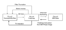
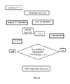
- FIG. 1 The T2*MRI and CIMRI model.
- the T2*MRI model is decomposed into two modules: “Source Magnetism” (in the upper dotted box) and “MRI technology” (in the lower dotted box).
- the downward arrows indicate the forward procedure and the upward arrows indicate the backward procedure.
- the CIMRI model consists of two steps as diagramed in the circle.
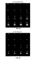
- FIG. 2 ( a ) A predefined 3D ⁇ distribution (16 z-slices of Gaussian blob), and (b) the magnitude image of the T2*MRI simulation.
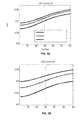
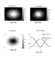
- FIG. 3 The spatial correlations between the T2*MRI magnitude (denoted by A) and the predefined ⁇ distribution for two intravoxel vasculatures (2-um-radius in (a 1 ) ( FIG. 3A ) and 4-um-radius in (a 2 )) ( FIG. 3B ) and for three voxel sizes (see legend).
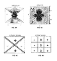
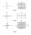
- FIG. 4 ( a ) Visualization of the 3D convolution kernel h 0 (x,y,z) with three isosurfaces at isovalues of ⁇ 0, 0.8, ⁇ 0.8 ⁇ ; (b) a 2D quadruple pattern at a longitudinal plane at h 0 (x,0,z); (c) a digital texture detector associated with (b); and (d) a standard 2D digital edge detector.
- the 3D h 0 (x,y,z) is interpreted as a 3D texture template, which can enhance edges and boundaries.
- FIG. 5 Demonstration of the morphormetric difference between a Gaussian-shaped ⁇ distribution in (a) and its fieldmap in (b).
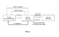
- FIG. 6 The CIMRI model (diagrammed with solid arrows). It consists of two inverse mappings: fieldmap calculation from MR phase image and ⁇ reconstruction from the fieldmap. There are three solvers for ⁇ reconstruction from fieldmap: filter truncation, matrix inverse, and TV iteration (our proposal). The forward MRI is diagrammed with rightward arrows.
- FIG. 7 ( a ) Precomputed fieldmap (resulting from a predefined neuroactive blob), and (b) the phase image of T2*MRI simulation. It is noted that the MR phase image can faithfully represent the fieldmap.
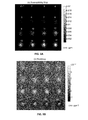
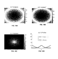
- FIG. 8 The spatial correlations between the MR phase image and the precomputed fieldmap (see FIG. 7 ) for two intravoxel vasculatures (2-um-radius in (a 1 ) ( FIG. 8A ) and 4-um-radius in (a 2 )) ( FIG. 8B ) and for three voxel sizes (see legend).
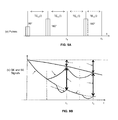
- FIG. 9 Illustration of T2′-effect signals with two echo times.
- T2* SE signal echoes in black
- T2* GE signal echoes in red.
- the T2* SE signals are generated by a pair of 90° and 180° pulses.
- the T2* GE signals are generated by only a 90° pulse and a reversal readout gradient (not drawn).
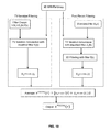
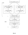
- FIG. 10 Feature-specified ⁇ reconstruction by “post-recon filtering” and “TV-iteration filtering” approaches.
- the “post-recon filtering” approach is carried out by first reconstructing a ⁇ source with standard TV iteration and then exerting a spatial filtering with a feature-specified filter ⁇ (k), as diagramed in the right-hand dotted box.
- Two approaches are carried out in parallel, and the two resultant ⁇ sources are averaged to produce a noise-reduced ⁇ source.
- FIG. 11 3D convolution filter design.
- a modified kernel can be obtained by DC term reset, lowpass, highpass, and bandstop filtering. (The bandpass filtering is not shown).
- FIG. 12 Demonstration of the equivalence of “TV-iteration filtering” and “post-recon filtering” and the noise reduction by average.
- the “post-recon filtering” with a lowpass filter ⁇ LP (k) [0.6+0.4 cos( ⁇ k/k max )];
- FIG. 13 The neighborhood of DC term of the standard filter H 0 (k).
- the profiles of the scanline (only provided in (a)) is shown in (d). It is seen that the DC value of H o (k) has little influence on TV-regularized ⁇ reconstruction (as described “scale invariance”).
- FIG. 15 Diagram for bandpass, highpass, and lowpass filtering which is applied to a direction along k x -, k y -, k g -axis, and radial direction k, separately and jointly.
- the red plots have sharp cutoffs and the black plots are smooth which can suppress Gibbs effect.
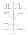
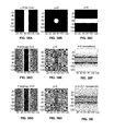
- FIG. 16 Illustrations of strip feature extraction by designing the filters for horizontal stripe extraction (at top row; FIG. 16A ), vertical stripe extraction (at middle row; FIG. 16B ), and the extraction for vertical, horizontal, diagonal, and anti-diagonal stripes (at bottom row; FIG. 16C ).
- the spatial superimposition of numerous random stripes makes a clutter noise in the reconstruction.
- FIG. 17D shows the 1D profiles of lowpass, hiqhpass, and lowpass squared filters.
- FIG. 18 The reciprocals of the filters in FIG. 17A-D are shown in FIG. 18A-D , respectively.
- the profiles of the scanline (indicated in (a)) are shown in (d).
- FIG. 20 A MR magnitude-based self-calibration scheme for estimating the TV regularization parameter value.
- the MR magnitude image is used as a reference to compare with the trial TV iteration outcome, thereby determining the initial guess of proper TV iteration parameter values for ⁇ reconstruction. It is noted that the magnitude is compared with the absolute value of susceptibility.
- FIG. 21 Noise reduction strategy by parallel TV iteration (using different parameter values) and multiple reconstruction average.
- FIG. 22 Demonstration of noise reduction by multi-recon average.
- the ⁇ reconstruction suffers sparse “residual noise” (or comeback noise associated with Bregman iteration), as indicated in dotted circles.
- the average of multiple reconstructions ((a 1 ) through (a 5 ) with different ⁇ values) FIG. 22A-E , respectively can effectively reduce the sparse noise as shown in (b) ( FIG. 22F ).
- FIG. 23 Profiles of scanlines in FIG. 22 .
- the amount of noises (calculated by standard deviation) are provided in the figure legend.
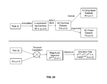
- FIG. 24 There are only three datasets available for a BOLD ⁇ MRI study ⁇ task(t), A(x,y,z,t), P(x,y,z,t) ⁇ .
- Lower box the neuroactive site in the FOV can be determined by the temporal correlation between the task(t) and magnitude timecourses.
- FIG. 25 4D susceptibility reconstruction under the criterion of susceptibility timecourse synchrony (a way of making use of the external stimulus paradigm task(t)), where tcorr(x(t),y(t)) stands for temporal correlation between x(t) and y(t).
- the neuroactive location (x act , y act , z act ) is determined in FIG. 24 .
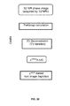
- FIG. 26 Structural ⁇ tomography scheme for susceptibility-based nonheme iron deposit measurement by structural MR imaging and CIMRI (toward applications for tissue and organ iron imaging).
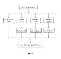
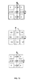
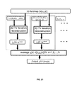
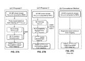
- FIG. 27 Two methods for susceptibility-based brain mapping and neuroimaging in (a 1 ) ( FIG. 27A ) and (a 2 ) ( FIG. 27B ), which are different from the conventional magnitude-based brain mapping and neuroimage in (b) ( FIG. 27C ).
- the method 1 in (a 1 ) ( FIG. 27A ) is for linear statistical data analysis
- the method 2 in (a 2 ) ( FIG. 27B ) is for nonlinear linear statistical analysis.
- FIG. 28 A method to improve the ⁇ tomography by T2′MRI and CIMRI.
- the Gradient-echo image and spin-echo image are acquired for the same ⁇ source with the same echo time T E .
- a complex division is used to obtain a complex T2′ complex image.
- a CIMRI analysis is used to reconstruct the susceptibility source from T2′ phase image.
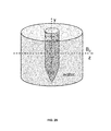
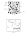
- FIG. 29 Gd-filled tube phantom experiment setup.
- the tube phantom provides a static cylindrical susceptibility distribution, which is used to simulate a snapshot of dynamic susceptibility-expressed physiological process.
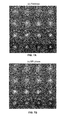
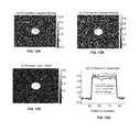
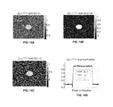
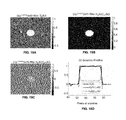
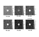
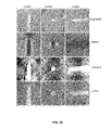
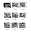
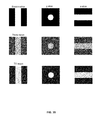
- FIG. 30 Phantom experiment results. Row 1 (at top): magnitude image; Row 2: phase image; Row 3: ⁇ reconstructed from filter truncation method; and Row 4 (at bottom): ⁇ reconstructed from TV iteration method.
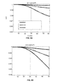
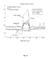
- FIG. 31 Quantitative profiles along a cylinder diameter in FIG. 30 .
- FIG. 32 TV-regularized brain ⁇ reconstruction from an in vivo experiment dataset.
- FIG. 32A an axial slice of the MR magnitude of brain imaging (where a vertical segment marks a scanline);
- B 1 FIG. 32B
- the phase image slice (b 2 ) ( FIG. 32C ) the smoothed phase;
- c 1 -c 6 ( FIG. 32D-I ) the ⁇ reconstruction from the phase (in (b 1 ; FIG. 32B )) by using a large range of ⁇ values.
- the magnitude image is nonnegative as displayed in a greyscale bar range of [0,1], and all other images (phase images and ⁇ reconstructions) are bipolar-valued.
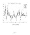
- the rectangle waveform represent the external stimulus task(t).
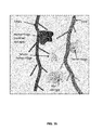
- FIG. 35 Illustration of brain structural susceptibility distribution.
- the hemorrhage and micro-hemorrhage of blood circulation causes spread susceptibility distribution, the static iron deposit also contributes the susceptibility distribution for static structural representation.
- the iron deposit may occur in tissues and organs, not necessary in proximity to blood streams.
- the static iron deposit in tissue and organ can be measured by 3D magnetic susceptibility tomography.
- FIGS. 36A and 36B Illustration of blood susceptibility perturbation associated with a BOLD ⁇ MRI model.
- the extravascular tissue is the static background structure.
- the BOLD-induced susceptibility perturbation is attributed to the intravascular blood-borne heme iron disturbance.
- the dynamic heme-iron perturbation, superimposed on a static structural iron background, can be measured by 4D magnetic susceptibility tomography.
- FIG. 37 Geometry for cylindrical ⁇ reconstruction numerical simulation. The main field is perpendicular to the cylinder.
- FIG. 39 Numerical simulation results of computed inverse BOLD ⁇ MRI for susceptibility source reconstruction with a simple cylinder ⁇ source (predefined ground truth in the first row), by filter truncation method (in second row) and by the TV-regularized method (in the third row).
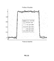
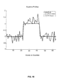
- FIG. 40 Quantitative profiles along a diameter of the cylinder phantom in FIG. 37 (the ground truth is a rectangle profile in legend “truth”).
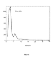
- FIG. 41 Convergence of a typical TV iteration.
- FIG. 42 Comparison of two inverse solvers in a numerical simulation of random noise behavior during ⁇ reconstruction.
- CIMRI Computed Inverse Magnetic Resonance Imaging. It is a computational model for reconstructing the magnetic susceptibility source of T2*MRI by reversing the forward MRI procedure by computations. It comprises two computation steps: fieldmap calculation from MR phase image and susceptibility calculation from the calculated fieldmap.
- the CIMRI provides a means for magnetic susceptibility tomography.
- 3D convolution magnetization When a foreign nonferrous material is introduced into a magnetic field, it is subject to a magnetization process (due to the material and field interaction), which can be described by a magnetic dipole model in the linear magnetization regime.
- a magnetization process due to the material and field interaction
- TV iteration Total Variation iteration (or TV regularization). It is an iteration procedure for finding the optimal solution that simultaneously minimizes the TV norm and data fidelity.
- this invention we generalized the TV iteration for conventional 2D image restoration to accommodate our 3D deconvolution ⁇ reconstruction (the core technology of CIMRI).
- Post-recon processing or Post-recon filtering This is a postpocessing step exerted on a reconstructed susceptibility distribution.
- Typical post-recon processing strategies include: low-pass, highpass, bandpass, bandstop filtering.
- Reciprocal filter The filter 1/ ⁇ (k) is called the reciprocal of the filter ⁇ (k). Reciprocal filter is also called an inverse filter.
- TV-iteration kernel design This term refers to the design of TV iteration convolution kernel h(r).
- h(r) h 0 (r)*IFT[1/ ⁇ (k)]
- h 0 (r) represents the magnetic dipole kernel
- ⁇ (k) the filter designed for post-recon filtering
- IFT the inverse Fourier transform
- Comeback noise or residual noise refers to the random and sparse noise that is brought back during TV iteration.
- the pattern and distribution of the comeback noise varies during TV iteration process and with the TV iteration setting. Two TV iterations with different parameter settings do not bring back the same noise pattern.
- the comeback noise is also called residual noise. Usually, the comeback noise randomly and sparsely emerges in uniform regions.
- Parallel TV iteration This term refers to performing multiple TV iterations on the same fieldmap dataset with different iteration parameter settings, which are carried out in a manner of parallel computations.
- parallel TV iteration for the purpose of average noise reduction via parallel computations.
- Multi-recon average multi-reconstruction average.
- the output of parallel TV iteration comprises a multitude of ⁇ reconstructions, which have different residual noise (or comeback noise). We average the multiple ⁇ reconstructions to make a so-called “multi-recon average”.
- the multi-recon average can reduce random sparse comeback noise (at the cost of performing multiple TV reconstructions).
- ⁇ tomography Based on the conclusion that the magnetic susceptibility property (denoted by ⁇ ) represents the underlying source of T2*MRI, and that the MR magnitude image is a distortedly transformed image of ⁇ (due to local average and nonlinearity of MRI detection).
- ⁇ tomography Magnetic susceptibility tomography
- ⁇ tomography refers to ⁇ tomographic reconstruction from T2*MRI data by CIMRI, and it is used interchangeably with the term “ ⁇ reconstruction”.
- Structural ⁇ tomography (3D ⁇ tomography).
- the structural ⁇ tomography provides a ⁇ distribution that is interpreted as iron deposit measurement for biological tissue and organs.
- a ⁇ distribution can be obtained by CIMRI from a complex MR image.
- the content of structural reconstructed ⁇ is mainly the static nonheme iron deposit in tissue or organ (the microbleeding is considered as static in relative to small T E ).
- Functional ⁇ tomography (4D ⁇ tomography). This term refers to as reconstructing the dynamic ⁇ perturbations (imposed on a background) from a 4D complex MR dataset (acquired by BOLD ⁇ MRI) by implementing snapshot ⁇ reconstruction by CIMRI.
- the content of reconstructed ⁇ at a snapshot time consists of both static nonheme iron deposit (background or baseline) and dynamic heme iron perturbation (due to brain functional activity).
- ⁇ -based functional imaging which replaces the MR image dataset with the reconstructed ⁇ dataset.
- the ⁇ -based functional imaging improves the neuroimage depiction, because the reconstructed ⁇ distribution is a more direct and truthful representative of the neuroactivity than the MR magnitude image.
- Timecourse synchrony This term refers to a synchronous response to an external stimulus paradigm.
- the MR signal is formed due to the neuroactive response to the external stimulation. Therefore, the signal timecourses are highly correlated with the stimulus timecourse (usually with a time lag of 2 to 4 seconds).
- the magnitude timecourse synchrony we can find the brain active site on the temporal correlation map (the conventional neuroimage depiction technique). Since the underlying source of BOLD ⁇ MRI signals is the susceptibility perturbation, it is understandable that the internal susceptibility perturbation should be synchronous to the external stimulation (with a time lag due to homodynamic response latency). Therefore, we developed a susceptibility synchrony criterion for reconstructing a meaningful 4D susceptibility dataset.
- the susceptibility timecourse from the reconstructed 4D susceptibility dataset at the neuroactive regions assumes a high correlation with the external stimulation (with a time lag), where the neuroactive site can be determined by finding the maxima at the 3D magnitude temporal correlation map.
- T2* gradient-echo imaging also T2* imaging.
- This term refers to acquiring a gradient-echo image, which consists of all the transverse dephasing contributions, including the inhomogeneous fieldmap T2′ effect, spin-spin interaction T2 effect, and the proton diffusion effect.
- the conventional EPI pulse sequence is an implementation of T2* imaging.
- T2′-effect phase image (or T2′ phase image).
- the T2′-effect phase image is calculated from T2′-effect complex image, which is in turn calculated from a pair comprising: a T2* GE complex image and a T2* SE complex image, by a complex division.
- T2′-effect fieldmap (or T2′ phase image).
- the T2′-effect fieldmap is proportional to the T2′-effect phase image by a constant factor.
- the T2′-effect fieldmap consists only of the static inhomogeneous fieldmap with the random T2 effect removed by the T2′-effect image scheme. Therefore, the T2′-effect fieldmap can be used for improving the ⁇ reconstruction fidelity.
- the word “image” (e.g., “a MR phase image”) is broadly defined as meaning “a 3D volumetric array (x,y,z) of voxel signal values, whose voxel values are measured at a single T E value” (i.e., multivoxels). Also, the words: “map”, “distribution”, “volume”, “data”, “3D image”, “3D map”, “3D distribution”, “3D volume”, “volumetric map”, “3D image dataset”, and “3D data”, are equivalent to, and interchangeable with, the word “image”, as it is defined above.
- 4D dataset refers to a timeseries of MR images with 3D space and 1D time, as denoted by (x,y,z,t).
- the output of T2*MRI is a 3D MR image
- the output of a BOLD ⁇ MRI study is a 4D dataset that consists of a timeseries of volumetric (3D MR) images captured by T2*MRI at each snapshot in time.
- the MRI technology is an excellent noninvasive imaging modality for biological soft tissue and physiological state imaging.
- the magnitude image of a MR complex image is used to represent a physiological state or a brain interior, whereas the phase image remains largely unused.
- the MR magnitude image is not an exact representation of the underlying susceptibility source, and that the MR phase appears textural, noisy, spatially blurred.
- Our invention makes use of MR phase image for the ⁇ source reconstruction.
- Relevant theory, models, algorithms are provided. The algorithm implementations are demonstrated with numerical simulations. Details about the parameter settings, and implementations of two numerical simulation examples are provided in Appendix A. A phantom experiment, and a real human brain imaging experiment, are presented later in separate sections.
- the multivoxel values that populate a 3D volumetric array (x,y,z) of multiple voxel signal values are measured at a single TE, using a complex EPI or EVI pulse sequence, after a RF pulse has been applied.
- CIMRI computed inverse magnetic resonance imaging
- the 3D ⁇ reconstruction algorithm involves a 3D ill-posed deconvolution, for which we developed a 3D total variation (TV) regularized iteration solver with an efficient implementation of split Bregman iteration [17, 21].
- TV 3D total variation
- the output is a 4D complex MR dataset; from which we can reconstruct a 4D ⁇ dataset by reconstructing each 3D snapshot volume with CIMRI (4D ⁇ tomography).
- the ⁇ tomography by CIMRI offers a quantitative interpretation of iron deposit in a tissue/organ physiological state, structural or functional, static or dynamic, patient (physiopathology) or healthy, human or animal.
- a reconstructed ⁇ volume for a static tissue/organ state is interpreted as iron deposit therein
- a reconstructed snapshot ⁇ volume in a dynamic BOLD process is interpreted as a composite of static brain structural iron deposit (baseline) and dynamic brain function heme-iron distribution (BOLD activity).
- the susceptibility distribution is the underlying source of T2*MRI, and it can represent a physiological state more directly than the MR magnitude image in the sense of its timing closeness and intactness (prior to T2*MRI scanning and being free from imaging transformations) [19]. Therefore, in this invention, we replace the MR image dataset with the reconstructed ⁇ source dataset for more direct and truthful structural and functional brain image depictions.
- Our CIMRI methods are based on the 3D volumetric MR image that may be acquired by stacking slices (as acquired by EPI for example) or preferably by volume imaging (as acquired by EVI for example).
- Our reconstruction algorithm is based on 3D volume image, not based on a 2D slice image or on a few number of individual voxels. Our methods do not involve the calculation of susceptibility gradient vector map.
- our CIMRI methods do not use a by-side phantom for MRI data acquisition, and our iterative susceptibility reconstruction algorithm is based on a 3D total-variation-regularized split Bregman iteration on the MR phase volume data per se, not involving by-side phantom data.
- the MR phase image is acquired by the conventional T2*MRI procedure (through the use of a standard 2D EPI sequence or a 3D EVI sequence), which is not involving a particular requirement for anisotropic diffusion imaging.
- T1 signal represents the longitudinal magnetization recovery after a stimulus of radio frequency (RF) pulse
- T2 signal represents the transverse magnetization dephasing due to random spin-spin interaction (even if in a homogenous field)
- T2* signal represents the total transverse magnetization dephasing in an inhomogeneous field, consisting of both the T2 random effect and the inhomogeneous field effect (T2′ effect).
- T2* signal is detected by gradient echo (GE) imaging, which is essentially a free induction decay signal (FID) reflecting the tissue media property.
- GE gradient echo
- FID free induction decay signal
- T2′ imaging scheme (by a complex division) that can provide a complex image due to static inhomogeneous field that excludes the unwanted random T2 effect (as well be reported later).
- T2*MRI forward ⁇ imaging
- a T2*MRI procedure acquires a complex MR image for the ⁇ source.
- the ⁇ source distribution can be reconstructed from the MR phase image by reversing the MRI procedure, as designated by CIMRI (computed inverse MRI) in FIG. 1 .
- the ⁇ expression for a brain functional process is a time-dependent 4D ⁇ dataset, ⁇ (x,y,z,t), which produces a complex-valued 4D MR image dataset by repeating the T2*MRI for each snapshot capture (as described by BOLD ⁇ MRI).
- snapshot ⁇ reconstruction thus implementing 4D ⁇ tomography.
- FIG. 1 shows the T2*MRI and CIMRI models.
- the T2*MRI model is decomposed into two modules: “Source Magnetism” (in the upper dotted box) and “MRI technology” (in the lower dotted box).
- the downward arrows indicate the forward procedure and the upward arrows indicate the backward procedure.
- the CIMRI model consists of two steps, as diagramed in the circle.
- the forward MRI procedure undergoes two steps.
- the first step is the fieldmap establishment by susceptibility magnetization in a main field B 0 , which can be expressed by a 3D convolution transformation [20]:
- B 0 denotes the main field, ⁇ (x,y,z) the noise, h 0 (x,y,z) (or h 0 (r)) the 3D convolution kernel, which is the magnetic response of a point magnetic dipole at the origin (
- the second forward step in FIG. 1 produces a complex-valued image by an intravoxel dephasing summation.
- the multivoxel image is formed by:
- the fieldmap establishment from susceptibility source by a 3D convolution in Eq. (2) is a linear and spatially spread transformation.
- the complex modulo and complex argument operations in Eq. (5) are nonlinear.
- the susceptibility source reconstruction from fieldmap is a linear deconvolution problem.
- the fieldmap In small angle regime (a linear phase approximation condition), the fieldmap is linearly related to the MR phase image[19, 39], which simplifies the fieldmap calculation in the first inverse step of CIMRI.
- the deconvolution of CIMRI is an ill-posed inverse problem that is a non-trivial task.
- the source of susceptibility distribution is attributed to the nonheme iron store, denoted by ⁇ struc (x,y,z).
- T2*MRI simulation can be considered as a snapshot capture of dynamic BOLD ⁇ MRI.
- corr ⁇ ( A , ⁇ ; T E ) cov ⁇ ⁇ A ⁇ ( : ; T E ) , ⁇ ⁇ ( : ) ⁇ std ⁇ ⁇ A ⁇ ( : ; T E ) ⁇ ⁇ std ⁇ ⁇ ⁇ ⁇ ( : ) ⁇ ( 10 )
- A(:;T E ) represents the lexicographically ordered 1D array of the 3D array A(x,y,z,;T E ), ⁇ (:) the 1D lexicographic array of ⁇ (x,y,z), coy the covariance, std the standard deviation.
- T E is retained as an explicit parameter to remind the T E -dependence of MR magnitude image.
- FIG. 2 shows (a) a predefined 3D ⁇ distribution (16 z-slices of Gaussian blob), and (b) the magnitude image of the T2*MRI simulation.
- FIG. 2 shows (a) a predefined 3D ⁇ distribution (16 z-slices of Gaussian blob), and (b) the magnitude image of the T2*MRI simulation.
- FIG. 3 shows the spatial correlations between the T2*MRI magnitude (denoted by A) and the predefined ⁇ distribution for two intravoxel vasculatures (2-um-radius in (a 1 ) and 4-um-radius in (a 2 )) and for three voxel sizes (see legend).
- the simulation results show that: 1) the pattern match between MR magnitude image and ⁇ source gives rise to a correlation about 0.90, which is affected by voxel size (image resolution), vessel size, and echo time; and 2) a long T E is preferred to reduce the mismatch.
- a texture enhancer can serve as an edge enhancer as well, as illustrated with a standard edge detector in FIG. 4( d ), but is not optimal for edge detection. That is, the 3D convolution with a bipolar-valued kernel plays a 3D spatial derivative to some extent.
- FIG. 4 shows: (a) visualization of the 3D convolution kernel h 0 (x,y,z) with three isosurfaces at isovalues of ⁇ 0, 0.8, ⁇ 0.8 ⁇ ; (b) a 2D quadruple pattern at a longitudinal plane at h 0 (x,0,z); (c) a digital texture detector associated with (b); and (d) a standard 2D digital edge detector.
- the 3D h 0 (x,y,z) is interpreted as a 3D texture template which can enhance edges and boundaries.
- the 3D convolution kernel in FIG. 4 is an unusual integral kernel because of its bipolar-valued multilobes, anisotropic spreading, and 3D zerosurface embedment.
- a convolution kernel for image blurring assumes a nonnegative distribution, like a Gaussian-shaped point spread function and a boxcar-shaped motion blurring function.
- FIG. 5 shows a demonstration of the morphormetric difference between a Gaussian-shaped ⁇ distribution in (a) and its fieldmap in (b).
- FIG. 1 we decompose a T2*MRI procedure into two modules and diagram the forward procedure by downward arrows and the inverse procedure by upward arrows.
- CIMRI indicated in a circle
- FIG. 6 shows the CIMRI model (diagrammed with solid arrows). It consists of two inverse mappings: fieldmap calculation from MR phase image and ⁇ reconstruction from the fieldmap.
- ⁇ reconstruction from fieldmap filter truncation, matrix inverse, and TV iteration (our proposal).
- the forward MRI is diagrammed with rightward arrows.
- corr ⁇ ( P , b ; T E ) cov ⁇ ⁇ P ⁇ ( : ; T E ) , b ⁇ ( : ) ⁇ std ⁇ ⁇ P ⁇ ( : ; T E ) ⁇ ⁇ std ⁇ ⁇ b ⁇ ( : ) ⁇ ( 12 )
- FIG. 7 shows (a) precomputed fieldmap (resulting from a predefined neuroactive blob), and (b) the phase image of T2*MRI simulation. It is noted that the MR phase image can faithfully represent the fieldmap.
- FIG. 8 shows the spatial correlations between the MR phase image and the precomputed fieldmap (see FIG. 7 ) for two intravoxel vasculatures (2-um-radius in (a 1 ) and 4-um-radius in (a 2 )) and for three voxel sizes (see legend).
- the three different 3D deconvolution solvers are diagrammed in FIG. 6 .
- the split Bregman TV iteration algorithm outperforms the others solvers in the following aspects: 1) It preserves edges; 2) It denoises the data such that there is no need to render image smoothing a priori (Note that the TV iteration method was originally developed for 2D image denoising and that smoothing is prone to suppress image features); 3) It can accommodate large 3D phase maps per se without a convolutional matrix conversion; and 4) It is an iteration algorithm that can produce a stable optimal restoration by avoiding the divide-by-zero problem, and in particular, the split Bregman iteration guarantees fast convergence.
- CIMRI volumetric susceptibility reconstruction from a MR phase volume.
- the MR phase volume can be obtained by stacking 2D slices acquired by an EPI sequence.
- the slice-stacked volume is anisotropic (in-plane resolution is different from the across-plane resolution).
- An isotropic volumetric SM reconstruction can be achieved by acquiring an isotropic MR phase volume with isotropic voxels at a zero oblique angle and with no inter-slice gap.
- EVI echo volume imaging
- TV total variation
- 2D image restoration including grayscale image and color vector image
- regular blurring kernel a centralized nonnegative distribution
- ⁇ ⁇ ⁇ TV ⁇ sup ⁇ ⁇ ⁇ ⁇ ⁇ ⁇ ⁇ ( r ) ⁇ ⁇ ⁇ g ⁇ ( r ) ⁇ d r , ⁇ g ⁇ ⁇ ⁇ 1 ⁇ ( 14 )
- g denotes a vector functional variable that is bounded by
- the TV norm is also given by
- ⁇ ⁇ ⁇ ( r ) min ⁇ ⁇ BV ⁇ ⁇ ⁇ ⁇ ( r ) ⁇ TV + ⁇ 2 ⁇ ⁇ B 0 ⁇ h 0 ⁇ ( r ) * ⁇ ⁇ ( r ) - b ⁇ ( r ) ⁇ 2 2 ( 16 )
- BV is a bounded variation function space
- ⁇ is the Lagrange multiplier or the regularization parameter.
- the TV regularization methodology lies in its searching over all possible distributions ( ⁇ BV) to find an optimal distribution ⁇ such that it minimizes the TV norm and the data fidelity error simultaneously.
- the algorithm implementation of Eq. (16) is nontrivial. Recently researches show that the TV iteration can be effectively implemented by a split Bregman algorithm [21, 44, 48, 49].
- the basic idea of the split Bregman algorithm is to transform a constrained optimization problem into a series of unconstrained subproblems; then to solve each subproblem by a Bregman-distance-based iteration.
- the Bregman distance in Eq. (17) can be thought of as the difference between the value of function J at point u and the value of the first-order Taylor expansion of J around point v evaluated at point u. It has been approved that the use of Bregman distance in Eq. (17) can ensure fast convergence.
- the “comeback noise” is sparse, which may vary from iteration to iteration.
- the parameters ⁇ ‘ ⁇ 1 ’, ‘ ⁇ 2 ’, ‘a 1 ’, ‘a 2 ’ ⁇ are introduced for algorithm implementation and fast convergence.
- the 3D convolution in Eq. (20), such as h* ⁇ can be implemented by 3D filtering in Fourier domain.
- the filter H(k) is not truncated at all, which is different from the inverse filtering solver with a truncated filter (“filter trunc” solver).
- the 3-subproblems are solved one at a time (with respect to one of ⁇ ‘d’, ‘v’, ‘ ⁇ ’ ⁇ while keeping the other two fixed).
- the split Bregman TV iteration algorithm for the minimization problem in Eq. (20) can be summarized by the following algorithm [17, 53]:
- T2′MRI T2′-effect magnetic resonance imaging
- T2* SE signal echoes in black
- T2* GE signal echoes in red
- the T2* SE signals are generated by a pair of 90° and 180° pulses.
- the T2* GE signals are generated by only a 90° pulse and a reversal readout gradient (not drawn).
- our T2′-effect imaging scheme in Eq. (27) can be extended to two echo times (T E1 and T E2 ), as illustrated in FIG. 9 . Because our T2′-effect imaging scheme by Eq. (27) is a complex image manipulation and it does not involves the calculations of the T2, T2* and T2′ parameters, we claim that our T2′-effect imaging scheme is quite different from the T2′ imaging technique as reported in [53]. More generally, the T2′MRI scheme can be extended to multi-echo imaging (with more than two echo times).
- the T2′MRI method cannot completely remove the random T2 and diffusion effects because of the imperfect repeatability of sheer randomness in two successive scans; on the other hand, the signals resulting from random T2 and diffusion effects are largely repeatable for different tissue types. Therefore, the T2′MRI method can remove the tissue-type-dependent T2 and diffusion effects.
- the spatial structure of an image can be characterized by its spatial frequency in Fourier domain and can be modified by spatial filtering with a spatial frequency filter.
- a 3D ⁇ distribution through a TV iteration with the standard kernel h 0 (r)
- the typical filtering schemes include lowpass (LP), highpass (HP), bandstop (BT), and bandpass (BP).
- LP lowpass
- HP highpass
- BT bandstop
- BP bandpass
- TV-iteration filtering approach
- post-recon filtering approach
- both “TV-iteration filtering” approach and the “post-recon filtering” approach can produce the same results because the TV iteration algorithm is a linear procedure which allows a linear spatial filtering to be inserted in the iteration process or to be exerted after the iteration reconstruction.
- FIG. 10 shows feature-specified ⁇ reconstruction by “post-recon filtering” and “TV-iteration filtering” approaches.
- the “post-recon filtering” approach is carried out by first reconstructing a ⁇ source with standard TV iteration and then exerting a spatial filtering with a feature-specified filter ⁇ (k), as diagramed in the right-hand dotted box.
- Two approaches are carried out in parallel, and the two resultant ⁇ sources are averaged to produce a noise-reduced ⁇ source.
- FIG. 11 The “filter design” part in the “TV-iteration filtering” approach (in the left-hand dotted box in FIG. 10 ) is drawn in FIG. 11 .
- FIG. 11 shows a scheme for 3D convolution filter design.
- a modified kernel can be obtained by DC term reset, lowpass, highpass, and bandstop filtering. (The bandpass filtering is not shown).
- the TV-iteration reconstruction with a modified filter of a scaled DC term will produce similar result that is different mainly by a scale of c, which we call “scale invariance” (a built-in functionality of TV-regularized iteration). Due to the comeback noise effect associated with the TV iteration, two TV iterations with different DC terms will produce similar results that are different by noise patterns (randomness and sparseness). Therefore, we can make use of this “scale invariance” phenomenon for noise reduction purpose (as will be addressed later). Numerical simulations of TV-iterated ⁇ reconstruction with a modified H 0 that are different in H 0 (0,0,0) value are demonstrated in FIG. 14 .
- the susceptibility source map can be reconstructed by a TV-regularized split Bregman iteration algorithm (see, e.g., Eq. (20)).
- the solution can be changed by using a new convolution kernel, h(r), that is a modification of the standard dipole kernel h 0 (r).
- h(r) that is a modification of the standard dipole kernel h 0 (r).
- ⁇ ⁇ 0 recon min d , v , ⁇ ⁇ ⁇ d ⁇ ( r ) ⁇ TV + ⁇ 2 ⁇ ⁇ B 0 ⁇ v - b ⁇ 2 2 + ⁇ 1 2 ⁇ ⁇ d - ⁇ ⁇ - a 1 ⁇ 2 2 + ⁇ 2 2 ⁇ ⁇ v - h 0 * ⁇ - a 2 ⁇ 2 2
- ⁇ recon min d , v , ⁇ ⁇ ⁇ d ⁇ ( r ) ⁇ TV + ⁇ 2 ⁇ ⁇ B 0 ⁇ v - b ⁇ 2 2 + ⁇ 1 2 ⁇ ⁇ d - ⁇ ⁇ - a 1 ⁇ 2 2 + ⁇ 2 2 ⁇ ⁇ v - h * ⁇ - a 2 ⁇ 2 2 ( 31 ) If ⁇ recon is more desirable than ⁇ 0 recon , then we can obtain ⁇ recon from ⁇ 0 recon by performing
- Eq. (32) a “post-recon filtering” because ⁇ recon is obtained by filtering the susceptibility source ⁇ 0 recon (that was reconstructed by using the standard kernel h 0 (r)).
- ⁇ recon can also be directly reconstructed from the fieldmap by using a modified filter H(k) (corresponding to a modified kernel h(r)). It can be shown that, the filter (or kernel) modification is given by
- FIG. 15 Some typical 1D filters are shown in FIG. 15 .
- FIG. 15 shows diagram for bandpass, highpass, and lowpass filtering, which is applied to a direction along k x -, k y -, k g -axis, and radial direction k, separately and jointly.
- the red plots have sharp cutoffs and the black plots are smooth, which can suppress Gibbs effect.
- 16 shows illustrations of stripe feature extraction by designing the filters for horizontal stripe extraction (at top row), vertical stripe extraction (at middle row), and the extraction for vertical, horizontal, diagonal, and anti-diagonal stripes (at bottom row).
- the superimposition of numerous random stripes manifests as a clutter noise in the ⁇ reconstructions.
- FIG. 17 we demonstrate (with a 2D slice display) a lowpass filter ⁇ LP (k) in (a), a squared lowpass filter ⁇ LP (k;2) in (b), and a highpass filter ⁇ HP (k) in (c), as well as 1D profiles.
- f BP ⁇ ( k ) 1 - exp ⁇ ( - ⁇ k ⁇ 2 2 ⁇ ⁇ 1 ⁇ k max 2 ) + exp ⁇ ( - ⁇ k ⁇ 2 2 ⁇ ⁇ 2 ⁇ k max 2 ) , ⁇ 1 > ⁇ 2 ( bandpass )
- f BT ⁇ ( k ) exp ⁇ ( - ⁇ k ⁇ 2 2 ⁇ ⁇ 1 ⁇ k max 2 ) - exp ⁇ ( - ⁇ k ⁇ 2 2 ⁇ ⁇ 2 ⁇ k max 2 ) , ⁇ 1 > ⁇ 2 ( bandstop ) ( 37 )
- ⁇ denotes the standard deviation of Gaussian distribution, which controls the shape of filter.
- the TV-regularized deconvolution algorithm in Eq. (16) involves a regularization parameter ⁇ , whose value should be preset for a TV iteration.
- ⁇ whose value should be preset for a TV iteration.
- ⁇ the proper values for ⁇ by comparing the iteration output with the predefined input (known).
- phantom experiment we can also compare the TV iteration output with the known phantom pattern, which is called system calibration in medical imaging.
- a phantom may be unavailable, or the magnetic susceptibility property of the phantom may deviate far differently from that of the imaging target. In such cases, especially for brain imaging where the brain interior susceptibility distribution remains unknown, we need find a way to estimate the TV iteration parameter value to ensure that the output of the TV iteration is a meaningful ⁇ reconstruction.
- FIG. 20 shows a magnitude-based self-calibration scheme for the TV regularization parameter value estimation.
- the MR magnitude image is used as a reference to compare with the trial TV iteration outcome, thereby determining the proper TV iteration parameter values for ⁇ reconstruction. It is noted that the magnitude is compared with the absolute value of the susceptibility value (which can be positive or negative valued).
- the “ ⁇ adjustment” box in FIG. 20 is for estimating an appropriate value, or a range, for the regularization parameter ⁇ , by using the MR magnitude image as a guide or an initial estimate of ⁇ source. Specifically, by comparing (usually by visual comparison) a reconstructed susceptibility source with the MR magnitude image during the trial iteration, we can estimate proper values for the TV regularization parameter. It is understandable that the MR magnitude image is not identical to the reconstructed susceptibility source (due to the magnitude's normegativity and T2*MRI nonlinearity). It is noted that we take into account the magnitude's non-negativity by comparing the magnitude image with the absolute value of reconstructed susceptibility.
- the TV iteration may bring back sparse noise in ⁇ reconstruction (see Eq. (19)).
- the comeback noise is different from the structure noise pattern in the fieldmap (phase image), that is, two iteration processes that are different by parameter settings may produce similar results that are different by residual noise pattern. Therefore, we developed a noise reduction strategy for ⁇ reconstruction by multiple TV iterations, followed by a multi-reconstruction average. Since different TV iterations can be carried out in parallel computation, we call it “parallel TV iterations”.
- parallel TV iterations By incorporating the DC term resetting approach, we implemented a parallel TV iteration scheme, as illustrated in FIG. 21 .
- FIG. 21 shows a noise reduction strategy by parallel TV iteration (using different parameter values) and multiple reconstruction average.
- the purpose of performing multiple ⁇ reconstructions by parallel TV iterations is for noise reduction by averaging.
- the TV regularization parameter ⁇ may assume a large range of values, typically from 20 to 1000, which is problem-specific. Therefore, a variety of ⁇ values can be used for TV iterations to produce a multiple of ⁇ reconstructions that are similar and different in residual noise. By averaging over the multiple ⁇ -variation ⁇ reconstructions, we obtain a noise-reduced ⁇ source.
- the ⁇ -varied ⁇ reconstructions can be used together with the scale-invariant ⁇ reconstructions (through resetting of DC term values).
- any and all of the variations of parameters ⁇ regularization ⁇ , DC term H 0 (0,0,0), auxiliary parameter ⁇ 1 and ⁇ 2 ⁇ can be used for multiple ⁇ reconstructions.
- the multiple reconstructions are carried out in parallel (at the cost of doing multiple computations). Then, the multi-reconstruction average is performed to produce a noise-reduced ⁇ source.
- the ⁇ reconstruction suffers sparse “residual noise” (or comeback noise associated with Bregman iteration), as indicated in dotted circles.
- the average of multiple reconstructions ((a 1 ) through (a 5 ) with different X values) can effectively reduce the noise, as shown in (b).
- Quantitative noise reductions and scanline profiles are shown in FIG. 23 .
- the noises (calculated by standard deviation) are provided in the figure's legend.
- TV iteration can reconstruct the susceptibility map with a powerful de-noising capacity, however, TV iteration may bring back sparse random noises in the uniform region of reconstructed susceptibility map (as demonstrated in simulations).
- the reconstructed susceptibility timecourse is synchronous with the stimulus task(t) with a lag time as well.
- timecourse synchrony between the timecourse of an observed image response or an reconstructed susceptibility perturbation and the designed stimulus task(t).
- the MR magnitude timecourse synchrony condition has been accepted for brain mapping and neuroimaging.
- FIG. 24 shows: Upper box: There are only three datasets available for a BOLD ⁇ MRI study ⁇ task(t), A(x,y,z,t), P(x,y,z,t) ⁇ . Lower box: the neuroactive site in the FOV can be determined by the temporal correlation between the task(t) and magnitude timecourses.
- ⁇ true (x,y,z,t) denote the dynamic can be predefined (as the ground truth) and the TV iteration reconstruction ⁇ *(x,y,z,t) can be compared with the truth thereby calibrating the parameter setting of ⁇ ‘ ⁇ ’,‘ ⁇ 1 ’ ‘ ⁇ 2 ’ ⁇ .
- the true susceptibility source is unknown (under investigation). It is the neuroimaging principle that the neuroimage can be inferred by observing the brain responses to a task paradigm (external stimulation). Given a task(t), we can find the neuroactive site in the cortical FOV by the local maximal temporal correlation as expressed by
- the active voxel in the susceptibility source is in the vicinity (neighborhood) of (x act ,y act ,z act ), denoted by neighbor(x act ,y act ,z act ), not necessarily at (x act ,y act ,z act ).
- neighbor(x act ,y act ,z act ) denoted by neighbor(x act ,y act ,z act )
- neighbor(x act ,y act ,z act ) not necessarily at (x act ,y act ,z act ).
- ⁇ recon ⁇ ( x , y , z , t ) max ( x ′ , y ′ , z ′ ) ⁇ neighbor ⁇ ( x act , y act , z act ) ⁇ ⁇ ⁇ ⁇ * ⁇ ( x ′ , y ′ , z ′ , t ) ⁇ ⁇ t ⁇ task ⁇ ( t ) ⁇ ⁇ ( 39 )
- ⁇ *(x,y,z,t) is a ⁇ reconstruction during program running for the snapshot time, t, by the TV-regularized split Bregman iteration algorithm (in Eq. (20)). The output in Eq.
- FIG. 25 shows a 4D susceptibility reconstruction under the criterion of susceptibility timecourse synchrony (a way of making use of the external stimulus task(t)), where tcorr(x(t),y(t)) stands for temporal correlation between x(t) and y(t).
- the neuroactive location (x act , y act , z act ) is determined in FIG. 24 .
- a proper ⁇ value for the TV reconstruction program should produce a voxel susceptibility timecourse at an active region such that it highly correlates (or anticorrelates) with the external task stimulus paradigm.
- the stimulus paradigm is widely used for postprocessing a BOLD ⁇ MRI dataset by SPM.
- T2*MRI is an inhomogeneous magnetic susceptibility distribution, which is mainly attributed to the iron content.
- the ⁇ distribution of an in vivo brain state consists of static nonheme iron deposit in tissue or organ structure and dynamic heme-iron perturbation in vascular blood associated with a brain functional activity.
- noninvasive iron measurement by CIMRI-based ⁇ tomography.
- tissue iron measurement we can perform 3D structural ⁇ tomography, and for dynamic functional heme-iron perturbation measurement, we can perform 4D functional ⁇ tomography (a timeseries of 3D ⁇ tomography).
- the origin of the structural susceptibility source is the nonheme iron deposit in tissues or organs, whereas the origin of the functional susceptibility source is the heme iron perturbation associated with vascular blood magnetism change caused by a functional activity (as described by the BOLD activity); and 2) the structural susceptibility distribution is static (bleeding is also considered as static in the sense that the bleeding motion is very slow in comparison with T E , that usually does not co-occur with the BOLD ⁇ MRI study) whereas the functional susceptibility perturbation is a dynamic response to a task paradigm. It is noted that a snapshot 3D volume in a 4D BOLD ⁇ MRI dataset consists of the contributions from both the static structural ⁇ background (baseline) and the dynamic functional ⁇ perturbation (activation).
- FIG. 26 we describe a structural ⁇ tomography scheme for the susceptibility-based nonheme iron measurement in tissues or organs.
- This scheme is characteristic of the following aspects: 1) It is 3D tomographic reconstruction of the structural ⁇ distribution (which is different from the voxel-based susceptometry or 2D image-based susceptibility mapping); and 2) The iron deposit image representation is based on the 3D ⁇ reconstruction by CIMRI from the 3D MR phase image, rather than from the MR magnitude image.
- FIG. 27 we describe two (new) ⁇ -based brain functional mapping schemes, as shown in (a 1 ) and (a 2 ), which are different from the conventional magnitude-based brain functional mapping method, as shown in FIG. 27( b ).
- the two new schemes in FIGS. 27( a 1 ) and ( a 2 ) are based on the ⁇ reconstruction.
- 27( a 1 ) is implemented by first calculating the phase-based brain activation map, denoted by P map (x,y,z), and then reconstructing the susceptibility-based activation map, ⁇ map (x,y,z) by performing CIMRI only once (the fieldmap b map (x,y,z) is calculated from P map (x,y,z) by using Eq. (13) and ⁇ map (x,y,z) is calculated from b map (x,y,z) by the TV-regularized split Bregman iteration scheme in Eq. (20)).
- the second (new) scheme in FIG. 27( a 2 ) is implemented by first reconstructing a 4D susceptibility dataset ⁇ recon (x,y,z,t) by looping the CIMRI for each time point of t, and then rendering the ⁇ -based statistical brain mapping. Both the first and second new schemes produce an output of ⁇ -based brain activation maps from a 4D BOLD ⁇ MRI dataset.
- the second scheme costs more computations than the first scheme; however, the second scheme can accommodate the nonlinearity of T2* phase image acquisition without a linear assumption for SPM and CIMRI.
- FIG. 27 shows our two new proposals of susceptibility-based brain mapping and neuroimaging in (a 1 ) & (a 2 ), which are different from the conventional magnitude-based brain mapping and neuroimage in (b).
- the proposal 1 in (a 1 ) is for linear statistical data analysis
- the proposal 2 in (a 2 ) is for nonlinear linear statistical analysis.
- the reconstructed 4D ⁇ dataset can represent the intrinsic neuroactivity more directly and veraciously than the 4D raw MR dataset (magnitude or phase), it is expected that the x-based brain mapping (proposal 2 in (a 2 )) and neuroimaging is more truthful than that based on the MR magnitude data.
- the proposal 2 in (a 2 ) can be implemented by the proposal 1 in (a 1 ) with reduced computations (performing CIMRI only once).
- the conventional BOLD ⁇ MRI data analysis tools such as SPM, independent component analysis (ICA), and connectivity graphs, can be applied to the 4D ⁇ dataset without change.
- the structural ⁇ tomography scheme provides a 3D ⁇ source for static iron deposit in tissues or organs (as illustrated schematically in FIG. 26 ).
- the functional ⁇ tomography scheme is to reconstruct a 4D ⁇ dataset (a dynamic ⁇ series), which is then used for brain mapping and neuroimaging, as illustrated schematically in FIG. 27 .
- the underlying source of a structural and functional state is the ⁇ distribution, which is mainly attributed to the iron origin; 2) the MR magnitude image suffers from a local average, and a nonlinear transformation of the ⁇ source; meaning that the MR magnitude image is not a tomographic reproduction of the ⁇ source; 3) the MR phase image is a linear transformation of the susceptibility source in the small angle regime (the 3D convolution is linear)) and the ⁇ source can be reconstructed from the MR phase image by CIMRI (by solving an ill-posed deconvolution); 4) if the statistical postprocessing is linear, it commutates with the CIMRI, thereby reducing the multiple CIMRI repetitions to a one-time CIMRI calculation.
- T2′-effect signal acquisition The principle of T2′-effect signal acquisition is illustrated in FIG. 9 , which aims to remove the random motion effect from the T2* signal.
- T2′-effect imaging we generalize this concept to the principle of T2′-effect imaging, as diagramed by T2′-effect MRI (T2′MRI) in FIG. 28 .
- T2′MRI T2′-effect MRI
- the T2′MRI procedure/analysis can be used to obtain a complex MR image (called T2′ complex image) that consists essentially of the static inhomogeneous field effect (e.g., the T2′ source).
- T2′ complex image consists essentially of the static inhomogeneous field effect (e.g., the T2′ source).
- T2′MRI procedure we perform CIMRI-based ⁇ reconstruction.
- FIG. 28 illustrates schematically the methodology to improve the ⁇ reconstruction, comprising (1) performing T2′MRI and then (2) CIMRI.
- the Gradient-Echo image and the Spin-Echo image are acquired from the same ⁇ source (i.e., the same object) with the same echo time, T E .
- a complex division is then used to obtain a complex T2′ image.
- a CIMRI procedure is used to reconstruct the susceptibility distribution from a T2′ phase image extracted from the T2′ complex image.
- the T2′MRI section in FIG. 28 consists of the following steps: 1) complex SE image acquisition by a spin-echo imaging with a T E ; 2) complex GE image acquisition by gradient-recall echo imaging, for the same ⁇ source with the same T E ; 3) T2′ complex image calculation by a complex division between the complex GE image and the complex SE image. From the T2′ complex image, we can calculate (extract) the T2′ phase image (by finding the complex argument), with which we can reconstruct the static susceptibility distribution by CIMRI by two steps: a) T2′ fieldmap calculation from the T2′ phase image and T E , and b) 3D static susceptibility reconstruction from the T2′ fieldmap.
- T2′ phase image is calculated by subtracting the T2 phase image from the T2* phase image (as presented earlier). Therefore, the inhomogeneous fieldmap associated with the T2 effect is greatly removed. Note that the method to improve the 3D ⁇ tomography by T2′MRI and CIMRI in FIG. 28 can be extended to 4D dynamic ⁇ tomography.
- the T2* GE image is acquired by an echo planar image (EPI) sequence; and the T2* SE image is acquired by a spin-echo EPI sequence.
- EPI echo planar image
- SE image is acquired by a spin-echo EPI sequence.
- the main difference between the pair of GE and SE pulse sequences is that the SE sequence includes an additional 180° pulse.
- the 3D complex image can be constructed by stacking the EPI slices.
- a 3D isotropic complex image may be directly acquired by an echo volumar imaging (EVI) sequence.
- An EVI sequence is used to acquire a 3D T2* GE complex image
- SE EVI sequence is used to acquire a 3D T2* SE complex image.
- the main difference between the EVI sequence and the SE EVI sequence is that the SE EVI includes an additional 180° pulse.
- the T2′MRI corrective procedure prefers a long T E due to the fact that a long T E causes a large T2 effect, and a large difference in T2* GE signal and T2* SE signal, and a large signal difference generally increases the digital subtraction stability and accuracy.
- a double-echo T2′-effect signal can be acquired by the illustration shown in FIG. 9 .
- the ⁇ tomography by our CIMRI model must be tested with phantom experiment before it can be used for practice.
- the trustworthiness of CIMRI-based ⁇ tomography is verified by having a successful comparison with a phantom experimental study.
- FIG. 29 shows a Gd-filled tube phantom experiment setup.
- the tube phantom provides a static cylindrical susceptibility distribution, which is used in simulations of a snapshot of dynamic susceptibility-expressed physiological process.
- FIG. 30 shows the experimental results of the MR magnitude, the MR phase, and the ⁇ tomographic reconstructions by both the “filter truncation” and “TV iteration” solvers.
- FIG. 30 shows the phantom experiment results.
- row 2 phase image
- row 3 ⁇ reconstructed from filter truncation method
- row 4 at bottom: ⁇ reconstructed from TV iteration method.
- FIG. 31 The quantitative profiles of scanline across a cylinder diameter are shown in FIG. 31 .
- the Gd-tube phantom experiment for CIMRI-based ⁇ tomography offers the following information: 1) The MR magnitude image suffers a central dip artifact; 2) The phase image is morphormetrically different from the ⁇ source due to the 3D convolution transformation in Eq. (2); 3) The ⁇ reconstruction by “filter truncation” method suffers strip artifacts and heavy noises; 4) the TV-iteration method can implement ⁇ tomography very well because the susceptibility source assumed an uniform distribution inside the cylinder, which agrees with the ‘ground truth’.
- a real brain imaging experiment was conducted with a healthy subject doing a finger-tapping visuomotor experiment in a Siemens Trio 3T scanner.
- a brain FOV was localized to cover the motor cortex part (the parietal lobe and frontal lobe in brain) with a 3D matrix in size of 90 ⁇ 90 ⁇ 30.
- the brain functional imaging experiment produced a 4D complex dataset (90 ⁇ 90 ⁇ 30 ⁇ 165 after image cropping) for a session of 330s scanning.
- the ⁇ reconstruction may take on a smoothing effect at a very small ⁇ ( ⁇ 30), and a contrast enhancement at a very large X (>500).
- FIG. 32 shows a TV-regularized brain ⁇ reconstruction from an in vivo experiment dataset, comprising: (a) an axial slice of the MR magnitude of brain imaging (where a vertical segment marks a scanline); (b 1 ) the phase image slice; (b 2 ) the smoothed phase; (c 1 -c 6 ) the ⁇ reconstruction from the phase (in (b 1 )) by using a large range of X values.
- the magnitude image is nonnegative as displayed in a greyscale bar range of [0,1], and all the images are bipolar-valued.
- FIG. 33 we plot the scanline profiles from FIG. 32( c 1 - c 6 ) for more quantitative inspection (the scanline was marked in FIG. 32( a )). It shows that the ⁇ reconstruction may suffer from oversmoothing effect for a very small ⁇ (e.g., 10), and from contrast enhancement for a very large ⁇ (e.g., ⁇ >1000). It also shows that the ⁇ reconstruction may assume similar reconstructions for an intermediate range of ⁇ values (e.g. in a range of 30-200)
- CIMRI models for reconstructing a 3D ⁇ source distribution from a 3D MR phase image acquired by T2*MRI, and for reconstructing a 4D ⁇ dataset from a 4D MR phase dataset.
- the former is mainly used for structural 3D ⁇ tomography and the later for functional 4D ⁇ tomography.
- Our structural 3D ⁇ tomography can be used for iron store measurement in organs (such as liver, spleen, pancreas, heart, brain) and in tissues (contrast agent and blood inside the vasculature, contrast and blood leakage, and in glands).
- organs such as liver, spleen, pancreas, heart, brain
- tissues contrast agent and blood inside the vasculature, contrast and blood leakage, and in glands.
- our method offers an accurate depiction of brain injury (hemorrhage, micro-hemorrhage, stroke) and brain dysfunctions (diseases).
- FIG. 35 we illustrate the ⁇ reconstruction for the image depiction of blood bleeding and microbleeding that occurs in the proximity of vasculatures.
- T2*MRI is widely used for imaging brain trauma, injury, and dysfunction
- our method provides a more truthful and accurate 3D tomographic image presentation of brain anatomical states in terms of reconstructed magnetic susceptibility.
- the reconstructed magnetic susceptibility can be interpreted as the iron deposit. Therefore our structural ⁇ tomography can find immediate use in iron deposit measurement of organs (liver, spleen, pancreas, heart, brain) and in tissues, not restricted the regions in the proximity of vasculatures.
- FIG. 35 shows an illustration of brain structural susceptibility distribution.
- the hemorrhage and micro-hemorrhage of blood circulation causes spread susceptibility distribution, the static iron deposit also contributes the susceptibility distribution for static structural representation.
- the iron deposit may occur in tissues and organs, not necessary in proximity to bloodstreams.
- Our 4D functional ⁇ tomography provides a susceptibility perturbation depiction for a neurovascular BOLD process (including a resting state, and a task-specific paradigm). Since a BOLD ⁇ MRI study produces a 4D complex dataset, our CIMRI produces a 4D dynamic susceptibility dataset accordingly.
- the functional ⁇ tomography together with statistical postprocessing, is useful for diagnostic and prognostic imaging of brain function diseases, such as schizophrenia, epilepsy, Alzheimer, aging, and other dysfunctions.
- FIG. 36 we illustrate the BOLD ⁇ MRI model for capturing the neurovascular-coupled BOLD states at the capillary bed.
- the intravascular blood susceptibility is perturbed by a functional activity, which may cause a negative susceptibility change in the arterial upstream (in artery and arterioles), a positive susceptibility change in capillary bed, and a positive susceptibility change in venous downstream (in venule and vein).
- the dominant heme iron susceptibility perturbation occurs in the capillary regions in response to the oxygen delivery and consumption, and the susceptibility perturbation in the arterial upstream is much smaller than that in the venous downstream.
- the BOLD ⁇ MRI is mainly attributed to the venous blood susceptibility. In such a case, the BOLD imaging is called a venography [2].
- FIG. 36 At the right-hand side in FIG. 36 is the conceptual illustration (a snapshot image) of susceptibility perturbation of intravascular blood and in extravascular tissue, which could be negative or positive.
- the positive and negative bipolar distributions are retained in the phase image, but not in the magnitude image because the magnitude image is a nonnegative representation [19] of a distribution that may consist of positive and negative values. Consequently, the negative susceptibility change will be inverted (called negative inversion) in the MR magnitude image because a magnitude value is nonnegative.
- the neuroactivity-caused susceptibility perturbation in terms of heme iron change is too weak to be perceived in a snapshot of MR image (with the background of structural ⁇ distribution).
- the BOLD activity can be extracted from a dynamic 4D dataset (acquired by ⁇ MRI under a task-specific paradigm) by a statistical postprocessing, such as a temporal correlation technique.
- FIG. 36 shows an illustration of blood susceptibility perturbation associated with a BOLD ⁇ MRI model.
- the extravascular tissue is the static background structure.
- the BOLD-induced susceptibility perturbation is attributed to the intravascular blood-borne heme iron disturbance. It is noted that the dynamic heme-iron perturbation is superimposed on the static structural iron background during MR image formation. In a single T2*MRI image, the contributions from the heme iron perturbation and non-heme iron deposit are inseparable.
- a preferred embodiment of a method of reconstructing an internal distribution (3D map) of magnetic susceptibility values, ⁇ ( x,y,z ), of an object, by using a Computed Inverse Magnetic Resonance Imaging (CIMRI) tomographic procedure, comprises the following steps:
- T E ⁇ 30 ms when performing functional MR imaging, and T E ⁇ 10 ms when performing structural MR imaging.
- the modified TV iteration filter, H(k) comprises one or more spatial processing capabilities selected from the group consisting of: lowpass, highpass, bandpass, and bandstop filtering.
- the 3D multiplier filter comprises radial symmetry or asymmetry, for a desirable susceptibility manipulation.
- the steps of estimating one or more appropriate values of the TV regularization parameter, ⁇ does not involve using an auxiliary phantom; so the selection of ⁇ is self-calibrated by using the accompanying MR magnitude information.
- the method comprises replacing the 3D T2*MRI phase image, P(x,y,z;T E ) in step b) of the preferred method above, with a 3D T2′-effect phase image, P T′ 2 (x,y,z;T E ); thereby improving the fidelity and accuracy of the reconstructed magnetic susceptibility map, ⁇ recon (r) by greatly reducing the T2 effect via MR phase angle subtraction (complex division).
- the T2′-effect MRI scheme is extended to multi-echo imaging comprising at least two different echo times, T E1 and T E2 .
- the T2′-effect MRI scheme is extended to multi-echo imaging by repeating echo planar image (EPI) sequences with multiple T E repetitions.
- EPI echo planar image
- the T2′-effect MRI scheme is extended to multi-echo imaging; wherein a 3D isotropic complex image is directly acquired by using an echo volumar imaging (EVI) sequence when imaging; and further wherein an EVI sequence acquires a 3D T2* GE complex image, while a SE EVI sequence acquires a 3D T2* SE complex image; wherein the main difference between the EVI sequence and the SE EVI sequence is that the SE EVI includes an additional 180° pulse for rephasing the non-random static dephasing.
- EVI echo volumar imaging
- the object comprises tissues or organs of a body; and wherein the method further comprises measuring a distribution of iron deposits in the tissues or organs of the body by interpreting the 3D reconstructed magnetic susceptibility map, ⁇ recon (r), as a quantitative distribution of iron deposits in said tissues or organs.
- the method does not comprise using any MR magnitude images; and further wherein the method does not comprise using any exponential decay parameters T1, T2, or T2*; or maps of said exponential decay parameters.
- Another embodiment of the present invention comprises a method of performing dynamic, magnetic susceptibility-based ⁇ MRI brain mapping and neuroimage depiction, using a MRI scanning machine, comprising: replacing a conventional 4D MR magnitude dataset (which is the conventional neuroimaging dataset) with a 4D reconstructed magnetic susceptibility dataset, ⁇ recon (r t); wherein r denotes 3D coordinates (x, y, z) in space domain, and t denotes a snapshot time.
- the 3D T2*MRI phase image, P(x,y,z;T E ), extracted in step b) comprises a wrapped phase image; in which case the preferred method described above further comprises generating a phase-unwrapped phase image, after step b), by performing a phase-unwrapping procedure on the wrapped phase image; followed by calculating the magnetic field map in step c), using the newly-generated phase-unwrapped phase image.
- a variety of means and methods can be used for displaying the results of the various method steps used in embodiments of the present invention, including, but not limited to: a) assigning either a gradation of grey values (greylevel bar), or a spectrum of color values (colorbar), to a selected 2D slice of data taken through the 3D map of reconstructed magnetic susceptibility values, ⁇ recon (r), thereby creating a 2D slice visual image representing a 2D distribution of reconstructed magnetic susceptibility values inside of the object; and, then b) displaying on a computer screen or monitor the resulting 2D slice visual image that represents a 2D distribution of reconstructed magnetic susceptibility values inside of the object.
- the 3D volume can also be displayed in 3D volume rendering or isosurface rendering.
- a 3D volume can also be display by a montage of 2D slices.
- the 4D dataset can be dynamically displayed with a video of 3D rendering.
- the methods and method steps, according to the present invention can be programmed in software in any efficient computer language (such as C, Matlab, Fortran, etc.) and be executed on desktop computers or higher workstations.
- any efficient computer language such as C, Matlab, Fortran, etc.
- Matlab language we implement our methods in Matlab language on a desktop computer: Intel® CoreTM 2 CPU 6600@ 2.40 GHz. 2.39 GHz, 2.00 GB of RAM).
- the algorithms can be implemented in multiple programs, which are arranged according the data flow (T2*MRI and CIMRI programs for numerical simulations, CIMRI programs for phantom and in vivo experiment). Each program is reserved some variables for the adjustable parameters (such as matrix size, newly designed kernel, regularization parameters) that are determined by problem-specific calibration. Based on data saving and reading operations, all the multiple programs can be organized into a single master program for a specific task, thus enabling program automation. The multiple programs can be executed independently on multiprocessors for parallel computations, also in automation (except for parameter adjustment and calibration).
- ⁇ ⁇ ( x , y , z ) ⁇ 1 inside ⁇ ⁇ cylinder 0 otherwise , ( x , y , z ) ⁇ FOV ( A1 )
- the parameter settings are provided in Table A1.
- FIG. 37 Geometry for cylindrical ⁇ reconstruction simulation.
- the main MR field is perpendicular to the cylinder's axis.
- the three orthogonal slices for the predefined ⁇ source and the calculated fieldmap (without and with noise) are displayed in FIG. 38 .
- FIG. 39 which compares the results of two different numerical simulations of computed inverse BOLD ⁇ MRI for susceptibility source reconstruction with a simple cylinder ⁇ source (predefined ground truth in the first row), by filter truncation method (in second row) and by the TV-regularized method (in the third row).
- FIG. 40 shows quantitative profiles along a diameter (scanline) of the cylinder phantom in FIG. 37 (note: the ground truth is a rectangle profile in legend “truth”).
- FIG. 41 shows the typical convergence behavior of the TV-iteration method. It is seen that the solution converges after about 15 iterations.
- the ⁇ tomography by “filter truncation” solver suffers from the heavy noise that manifests as the stripes and textural patterns [17,21-25], which is also demonstrated in FIG. 40 for the digital cylinder phantom simulation.
- the noise structure associated with the “filter truncation” solver can be explained by the illustration in FIG. 16 , wherein any two points in the Fourier domain creates a collection of parallel lines in the space domain, and the superimposition of a multitude of random parallel lines resulting from many random points in the Fourier domain manifests as a clutter noise or textural noise.
- the ⁇ tomography by “TV iteration” solver suffers only from sparse “comeback” noise [45-50].
Abstract
Description
-
- 3D: three dimension: (x,y,z)
- 4D: four dimension: (x,y,z,t)
- MR: Magnetic Resonance
- MRI: Magnetic Resonance Imaging
- T2*MRI: T2*-weighted MRI
- CIMRI: Computed Inverse MRI
- ƒMRI: functional MRI
- FID: Free Induction Decay.
- B0: main magnetic field
- TE, TE: Echo Time for both spin echo and gradient echo signals
- FOV: Field Of View
- NAB: NeuroActive Blob
- T1 relaxation: Longitudinal magnetization recovery process due to spin-lattice interaction.
- T2 relaxation (T2 effect): Transverse magnetization dephasing process due to random spin-spin interaction. (non-refocusable).
- T2′ relaxation (T2′ relaxation): Transverse magnetization dephasing process due to static field inhomogeneity. (refocusable).
- T2* relaxation: Total transverse magnetization dephasing process, consisting of T2 effect, T2′ effect, and diffusion effect. (partially refocusable).
- T2′ image: A complex image that is calculated by a complex division of a pair of T2* gradient-echo and spin-echo complex images.
- T2′ phase image: the phase part of T2′-effect complex image
- T2′ fieldmap: the fieldmap calculated from a T2′-effect phase image
- SE: Spin Echo
- GE: Gradient Echo.
- EPI: Echo Planar Imaging
- EVI: Echo Volume Imaging
- BOLD: Blood Oxygenation Level Dependent
- TV: Total Variation
- DC: Direct Current (electrical engineering term)
- FT: Fourier Transformation
- IFT: Inverse Fourier Transformation
- HP: HighPass
- LP: Lowpass
- BP: BandPass
- BT: BandStop
- trunc: truncation
- struc: structural
- conv: convolution
- recon: reconstruction
- r=(x,y,z): 3D coordinates in space domain
- k=(kx,ky,kz): 3D coordinates in Fourier domain (k-space)
- kmax=max{|k|}: the maximum modulus of k.
- χ tomography: a technique to reproduce an internal magnetic χ distribution from external measurement data.
- χ reconstruction: reconstructing a magnetic χ distribution from a MR phase image.
- χ0 (r): χ reconstruction with magnetic dipole model (χ0(k) in Fourier domain).
- χ(r): χ source, or processed χ, or χ reconstruction with modified kernel (χ(k) in Fourier domain).
- Δχ(r): susceptibility perturbation in reference to the baseline.
- b(r): 3D fieldmap (b(k)=FT[b(r)] in Fourier domain)
- h0(r): point magnetic dipole field (standard 3D convolution kernel).
- H0(k)≡FT[h0(r)]: standard χ reconstruction filter.
- ƒ(k): filter for post-recon χ filtering (as used by χ(k)=χ0(k)·ƒ(k)) in Fourier domain).
- H(k): modified deconvolution filter (H(k)=H0(k)/ƒ(k)=FT[h(r)] in Fourier domain
- h(r): modified deconvolution kernel (as formed by h(r)=h0(r)*FT[1/ƒ(k)])
- ε(r) Gaussian additive noise (ε(k) in Fourier domain).
- ∥χ∥TV: TV norm of χ.
- |C|: taking absolute value of C (complex modulo operation)
- ∠C: taking phase angle of a complex number C (complex argument operation)
- λ: TV regularization parameter.
- γ1, γ2: auxiliary parameters of TV iteration
- Ω(x, y, z): voxel at (x, y, z).
- |Ω(x, y, z)|: voxel size (=d0×d0×d0) (MR image resolution)
- c, c0, c1, c2: constants.
- ε0: a threshold for filter truncation (0<ε0<<1).
-
- Magnetic susceptibility tomography. Reconstruction of internal magnetic susceptibility distribution of an entity through the use of external MR measurement. The magnetic susceptibility tomography can be implemented by a computed inverse magnetic resonance imaging (CIMRI) model.
-
- Small angle regime. This term refers to a spin precession angle that is very small, such that exp(−iφ)˜1−iφ, with φ=γ·b·TE (Larmor law), where: γ denotes gyromagnetic ratio, b the magnetic field disturbance (the main field B0 is excluded in the rotating frame representation), and TE the precession time (or relaxation time, or echo time in a gradient echo sequence). In small angle regime, the fieldmap and MR phase image are different only by a TE-dependent scale factor. The condition of small angle regime can be reached by MR scanning with a small TE in a low field.
-
- TV-iteration convolution. This term refers to a TV iteration process that uses a modified convolution kernel (based on h0(r)). During a TV iteration process, each iteration is carried out by a 3D convolution with the same convolution kernel h(r) (a modification of h0(r)) and TV regularized minimization. Based on linear filtering theory, we show that a spatial filtering exerted on a 3D reconstructed χ (as described by post-recon filtering) can be equivalently achieved during TV iteration using a modified kernel.
- TV-iteration filtering. In practice, the 3D TV-iteration convolution can be efficiently implemented by performing the 3D iteration convolution part using 3D iteration filtering in the Fourier domain. Let h(r) represents the TV-iteration convolution kernel, the TV-iteration filter H(k) is calculated by H(k)=FT[h(r)], where FT stands for Fourier transform.
-
- T2* spin-echo imaging (e.g. T2 imaging). This term refers to acquiring a spin-echo image that only captures the T2 and diffusion random effects, with the static inhomogeneity dephasing canceled by 180° pulse refocusing. T2* spin-echo imaging is always called “T2 imaging”. We describe T2 image by a different name of “T2* spin-echo imaging” and use it to make a pair of T2* gradient-echo and spin-echo images.
- T2′-effect imaging (T2′MRI). We invented this scheme to obtain a complex image that consists of only static (non-random) inhomogeneous field effect (the T2′ effect). The T2′-effect imaging algorithm produces a complex image by a complex division of a T2* GE complex image divided by a T2* SE complex image. The output of T2′-effect imaging, denoted by T2′MRI, is not a map of T2′ parameter, so our T2′-effect image scheme is different from the T2′ imaging scheme. That is, T2′MRI is different from the conventional T2′ imaging in that: T2′MRI deals with the MR images per se, not involving the calculation of T2′ decay parameters for T2′ imaging.
-
- MR Signal. Traditionally, a MR signal refers to the free induction decay (FID) behavior of proton spin precessions with respect to relaxation time. In the context of MRI, a MR signal refers to the FID of a specific voxel with respect to the echo time TE. A MR image is a multivoxel array whose voxel values assume the voxel signals at a single value of TE. Both the MR voxel signal and MR multivoxel image are complex-valued in nature. In this invention, we do not need to perform MR signal observation. Instead, we involve MR multivoxel image capture by T2*MRI with a single echo time TE (or a few of TE's).
-
- 1. We describe the fieldmap establishment from a 3D χ source via magnetization in a main field by a 3D convolution model, which offers two advantages: explanation of the morphological mismatch between the χ source and the fieldmap (corresponding to phase image), and implementation of 3D χ tomographic reconstruction in the framework of 3D-deconvolution image restoration.
- 2. We solve the ill-posed 3D deconvolution problem associated with the 3D χ source tomography by a novel and unique 3D split-Bregman TV-regularized iteration method; for which we also developed a self-calibration scheme that selects the regularization parameter values (usually a range of values) by making use of the MR magnitude image to as an initial estimate of χ reconstruction.
- 3. We developed an improved TV-iteration filtering scheme by using a modified TV iteration filter that can achieve the similar results of spatial post-reconstruction filtering.
- 4. We discovered that the TV iteration is almost invariant to a wide range of TV regularization parameter values, and it is almost invariant to DC term reset. However, the TV iteration may bring back sparse noise in the uniform regions. We developed a noise reduction strategy by performing parallel TV iteration reconstructions (for the same fieldmap dataset but using different iteration parameter values), followed by a multi-reconstruction average.
- 5. We generate a 4D χ dataset from a 4D complex MR dataset (acquired by BOLD ƒMRI) by reconstructing each snapshot susceptibility volume from a MR phase volume in the 4D complex MR dataset by CIMRI. In order to make use of the external stimulus paradigm, we developed a criterion of susceptibility timecourse synchrony: the reconstructed susceptibility timecourse at the brain active site should maximally correlate with the timecourse of external stimulation.
- 6. We developed a unique T2′-effect imaging scheme to remove the random T2 and diffusion effects by acquiring a pair of T2* gradient-echo and spin-echo complex images and processing them by an element-wise complex division. By calculating the T2′ phase image from a T2′ complex image and using it for χ reconstruction, we can improve the χ reconstruction fidelity. Our T2′-effect imaging scheme does not involve exponential decay assumption, or the calculation for T2, T2* and T2′ parameters.
- 7. For applications, we developed a brain structural χ tomography scheme for nonheme-iron deposit measurement in tissue and organs, and a brain functional χ tomography scheme for heme-iron perturbation measurement for brain mapping and neuroimaging.
M z(t)=M z(t=0)(1−exp(−t/T 1))
M ⊥(t)=M ⊥(t=0)exp(−t/T 2)(in homogeneous field)
M ⊥(t)=M ⊥(t=0)exp(−t/T 2*)(in inhomogeneous field) (1)
with 1/T2*=1/T2+1/T2′
where B0 denotes the main field, ε(x,y,z) the noise, h0(x,y,z) (or h0(r)) the 3D convolution kernel, which is the magnetic response of a point magnetic dipole at the origin (as described by point magnetic dipole model). In Fourier domain, the 3D convolution is represented by a 3D filtering, that is:
where FT denoted Fourier transform, and H0(kx,ky,kz) the 3D filter (also denoted by H0(k), called standard filter) corresponding to the convolution kernel h0(x,y,z) in Eq. (2). It is noted that the DC term H0(0,0,0) is undefined due to a term of 0/0 (at kx=0, ky=0, kz=0), which allows to reset it (as will be shown later).
where γ denotes the proton gyromagnetic ratio, TE denotes the echo time (interpreted as an exposure time of T2*MRI), and χ(x,y,z) denotes the voxel at (x,y,z), and |Ω| the voxel size.
The magnitude image A(x,y,z) represents the 3D map of signal loss (decay), and the phase image P(x,y,z) the phase angle accumulation during TE (decay signals in reference to non-decay signals at TE=0).
C(T E)=C(T E=0)exp(−T E /T2*)(exponential decay model)
A(T E)=1−exp(−T E /T2*)(expoenetial magnitude loss) (6)
with which other researchers have used for T2*-based susceptibility mapping [3, 5, 6, 34-38]. It is noted that, in this report, we do not involve the exponential assumptions in Eq. (6) at all, and we only deal with the 3D T2*-effect images in Eq. (5). Therefore, we claim that our method is dealing with the T2 and T2* images per se, which is different from the T2 and T2*(or R2 and R2*) MR imaging techniques that involve the exponential models and decay rate calculation (requiring multi-time image acquisition through the use of a multi-echo sequence).
χtotal(x,y,z,t)=χstruc(x,y,z)+χfunc(x,y,z,t) (7)
where the time-dependent susceptibility χfunc(x,y,z,t) is due to the neurovascular-coupled BOLD process. We express the susceptibility dynamics associated with a BOLD activity by [18, 40]
χfunc(x,y,z,t)=x blood ·V(x,y,z)·NAB(x,y,z,t)
χblood =Hct·χ RBC+(1−Hct)·χplasma
χRBC=χoxy+(χdeoxy−χoxy)·(1−Y) (8)
where Y denotes oxygenation level, Hct the blood hematocrit, V(x,y,z) the vasculature-filled region, NAB(x,y,z,t) the neuroactive blob which is modulated by the external stimulation, χplasma the magnetic susceptibility of blood plasma, χoxy the magnetic susceptibility of oxyhemoglobin, and χdeoxy the magnetic susceptibility of deoxyhemoglobin with χdeoxy−χoxy=0.27×4π×10−6 (SI unit). For a BOLD process, we represent a BOLD state in terms of susceptibility perturbation in reference to a baseline state, denoted by Δχ(x,y,z,t), as expressed by
Δχ(x,y,z,t)≡(χdeoxy−χoxy)(1−Y)·Hct·V(x,y,z)·NAB(x,y,z,t) (9)
The susceptibility perturbation due to a functional activity is the underlying source of BOLD ƒMRI. Therefore, we can consider the BOLD ƒMRI as an application of T2*MRI technology to dynamic functional imaging by repeating the T2*MRI procedure for a timeseries of snapshot captures. It is noted that the 4D dataset represents a timeseries of 3D snapshot volumes.
Mismatch Between MR Magnitude Image and χ Source
where A(:;TE) represents the lexicographically ordered 1D array of the 3D array A(x,y,z,;TE), χ(:) the 1D lexicographic array of χ(x,y,z), coy the covariance, std the standard deviation. In Eq. (10), TE is retained as an explicit parameter to remind the TE-dependence of MR magnitude image. This correlation for matching two patterns is invariant to grayscale normalization (peak=1 is not required), and it produces a value for matching goodness in a range from 0 (completely different) to 1 (perfect matching with a difference of constant factor).
where H0(kx,ky,kz) is the Fourier transform of h0(x,y,z) (defined in Eq. (3)). Usually the DC term of the standard 3D filter H0(kx, ky, ky) assumes H0(0,0,0)=1/3 (when 0/0=0 is used in Eq. (11)). From the viewpoint of image processing [43], a convolution kernel h0(x,y,z) that possesses the properties in Eq. (11) serves as a 3D texture enhancer (H0(0,0,0)=0 for texture detector). In
-
- 1) It is of 3D spread distribution (not a point delta function), which explains the non-local property of the fieldmap and MRI phase image.
- 2) It is a 3D bipolar-valued kernel (not a unimode distribution like a Gaussian shape) and it manifests a 3D texture enhancer as understandable from Eq. (11) and
FIGS. 4( b) and (c). Therefore, it is not surprising that the phase image appears noisy. It is noted that the fieldmap of a uniform χ distribution will be reduced by a factor of ⅓ (=H0(0,0,0)) during the convolutional magnetization. - 3) It bears a 3D zerosurface for h0(r)=0 (see
FIGS. 4( a) and (c)), which means the deconvolution is an ill-posed inverse problem. - 4) It is anisotropic, which explains the orientation dependence in fieldmap and MRI image.
- 5) It is of radial symmetry about the origin and revolution symmetry about z-axis (see
FIG. 4( a)).
-
-
Step 1. Fieldmap establishment b(x,y,z) by magnetization of the susceptibility distribution x(x,y,z) in a main field B0, as expressed by Eq. (2). -
Step 2. Complex-valued image generation C(x,y,z) by intravoxel dephasing, as expressed by (Eq. (4)).
From the complex image, we obtain the magnitude image and phase image by Eq. (5). We reconstruct the χ source by a CIMRI model inFIG. 6 . Reversing the forward MRI procedure, the CIMRI consists of two inverse mappings: (i) fieldmap calculation from MR phase image, (ii) χ calculation from fieldmap. The two inverse mapping steps are addressed below with a numerical simulation.
Inverse Step 1: From MR Phase Image to Fieldmap
-
b(x,y,z;T E)=c·P(x,y,z;T E)with c=const(in small angle regime) (13)
-
- Solver Type 1: 3D filter truncation. This method suffers stripe effect and image energy shift.
- Solver Type 2: Matrix inverse. This method is limited by a dimensionality curse, that is, it cannot accommodate a large 3D matrix. (a small 3D matrix, say 16×16×16, cannot offer meaningful image features in a large FOV).
-
Solver Type 3. 3D TV iteration (our preferred method). This method can produce an excellent image restoration without the sufferings as confronted in previous two methods. The theory, algorithm, and implementation are addressed below.
where g denotes a vector functional variable that is bounded by |g|≦1. Strictly speaking, ∥χ∥TV is a semi-norm for that ∥χ∥TV=0 is allowed for χ≠0. For a smooth 3D function χ(r), the TV norm is also given by
where BV is a bounded variation function space, and λ is the Lagrange multiplier or the regularization parameter. The TV regularization methodology lies in its searching over all possible distributions (χεBV) to find an optimal distribution χ^ such that it minimizes the TV norm and the data fidelity error simultaneously.
D J(u,v)=J(u)−J(v)−<∂J(v),u−v> (17)
where the bracket <,> represent inner product, ∂J(v) is an element of the subgradient of function J at v. Intuitively, the Bregman distance in Eq. (17) can be thought of as the difference between the value of function J at point u and the value of the first-order Taylor expansion of J around point v evaluated at point u. It has been approved that the use of Bregman distance in Eq. (17) can ensure fast convergence.
where the parameters {‘γ1’, ‘γ2’, ‘a1’, ‘a2’} are introduced for algorithm implementation and fast convergence. It is noted that the 3D convolution in Eq. (20), such as h*χ, can be implemented by 3D filtering in Fourier domain. However, the filter H(k) is not truncated at all, which is different from the inverse filtering solver with a truncated filter (“filter trunc” solver).
b T
It is known that the static dephasing is refocusable by a 180° pulse, and that the dynamic dephasing associated with the random spin-spin interaction and diffusion motion are non-refocusable. We can describe these facts by
b T′2(x,y,z)=b T′2(x(t),y(t),z(t))=b T′2(x(t+T E/2),y(t+T E/2),z(t+T E/2))(refocusable)
b T
b diffu(x(t),y(t),z(t))≠b diffu(x(t+T E/2),y(t+T E/2),z(t+T E/2)(non-refocusable) (24)
Then, the complex SE image is expressed by
Obviously, for a special deal case in absence of dynamic T2 random effects and diffusion effects, the T2* SE refocusing gives rise to
Since the T2* GE signal consists of both the T2 effect (random spin-spin interaction and spin diffusion) and T2′ effect (static inhomogeneous field) and the T2* SE signal only consists of non-refocusable random T2 effect (that is, the T2* SE signal is the T2-effect signal), it is possible the separate the T2′-effect signal from T2* GE signal by signal decomposition. Concerning the fact that we are dealing with complex-valued MR images, we use complex division to calculate the T2′-effect complex image, as given by
C T′
which is called T2′-effect imaging scheme.
Therefore the magnitude behavior in Eq. (28) is compatible with the exponential signal intensity decay model [2]. It is seen in Eq. (28) that the maps of T2, T2* and T2′ can be calculated by exponentially fitting each voxel intensity decay. The connotations of T2, T2* and T2′ values for voxel signal intensity decays are illustrated in
It is expected that the T2′ complex image will greatly remove the T2 effect and diffusion effect (albeit incomplete due to imperfect repeatability of random effect in two different times), thereby improving the χ reconstruction fidelity. In principle, our T2′-effect imaging scheme in Eq. (27) can be extended to two echo times (TE1 and TE2), as illustrated in
This indicates that if the DC term H0(0,0,0) is modified by a multiplicative constant, c, it is equivalent to multiplying the kernel by the same constant. In other words, the TV-iteration reconstruction with a modified filter of a scaled DC term will produce similar result that is different mainly by a scale of c, which we call “scale invariance” (a built-in functionality of TV-regularized iteration). Due to the comeback noise effect associated with the TV iteration, two TV iterations with different DC terms will produce similar results that are different by noise patterns (randomness and sparseness). Therefore, we can make use of this “scale invariance” phenomenon for noise reduction purpose (as will be addressed later). Numerical simulations of TV-iterated χ reconstruction with a modified H0 that are different in H0(0,0,0) value are demonstrated in
If χrecon is more desirable than χ0 recon, then we can obtain χrecon from χ0 recon by performing a 3D spatial filtering with a filter ƒ(k) (or by a 3D convolution with a kernel ƒ(r)), that is
χrecon(k)=χ0 recon(k)·ƒ(k)(3D filtering)
or χrecon(r)=χ0 recon(r)*ƒ(r)(3D convolution) (32)
where IFT denotes Inverse Fourier Transform. When the modified filter H(k) obtained in Eq. (33) is used in the 3D susceptibility reconstruction by the TV iteration in Eq. (31), we say that the 3D susceptibility is reconstructed by a “TV-iteration filtering”. We will show that the TV-regularized iteration convolution scheme using a new kernel h(r) (corresponding to TV-iteration filtering using a new filter H(k)) (in Eq. (33)) to reconstruct a susceptibility source χrecon by Eq. (31), such that is has the same features as resulting from post-recon filtering using a filter ƒ(k) in Eq. (32).
ƒLP(k)=c 1 c 2×cos(πk/k max)s.t. min{ƒLP(k)}>0
ƒLP(k)=0.6+0.4×cos(πk/k max)(case: c 1=0.6 and c 20.4) (34)
with kmax=max {|k|}
The condition for a lowpass filter is min{ƒLP(k)}>0, as required by the non-singularity of 1/ƒLP(k). In Eq. (34), we provide a special case of c1=0.6 and c2=0.4, which produces min{ƒLP(k)}=0.2.
ƒHP(k)=max(ƒLP)−ƒLP(k)+c 0 s.t. min {ƒHP(k)}>0
ƒ HP(k)=max(ƒLP)−ƒLP(k)+0.2(case: c 0=0.2) (35)
As required by 1/ƒHP(k), we impose the highpass filter a condition of min{ƒLP(k)}>0. In Eq. (35), we also provide a special case of c0=0.2 such that min{ƒLP(k)}=0.2.
ƒLP(k;α)≡[ƒLP(k)]α, α={½,1,2,3 . . . }
ƒHp(k;α)≡[ƒHP(k)]α, α={½,1,2,3 . . . } (36)
It is noted that the filter shape can be dilated with 0≦α≦1 and shrunk with α>1. In this way, we can design different lowpass and highpass filters by selecting proper values for the parameters of {c0,c1,c2,α}.
where σ denotes the standard deviation of Gaussian distribution, which controls the shape of filter. Based on our numerical simulations, we find that the bandstop and bandpass filtering is useful for high spatial resolution χ reconstruction.
where χ*(x,y,z,t) is a χ reconstruction during program running for the snapshot time, t, by the TV-regularized split Bregman iteration algorithm (in Eq. (20)). The output in Eq. (39) is an optimal χ reconstruction under the criterion of susceptibility synchrony by varying the TV regularization parameter. In algorithm implementation, the λ-adjustment is continued until the 4D susceptibility source reconstruction produces a highest-as-possible temporal correlation between the timecourse at an activation voxel and the external stimulation. The strategy is diagrammed in
χmap(x,y,z)=SPM{χrecon(x,y,z,t),task(t)}(definition)
=SPM{CIMRI{P(x,y,z,t)},task(t)}(proposal 2)
CIMRI{SPM{P(x,y,z,t),task(t)}}(linear commutation)
=CIMRI{P map(x,y,z)}(proposal 1) (40)
-
- 1) The χ reconstruction with a very small λ (=10) could not restore the rectangular stimulus paradigm,
- 2) The χ reconstruction with a very large λ (=1000) could not restore the rectangular stimulus paradigm either,
- 3) The χ reconstruction with a range of λ values ([20-500]) could restore the rectangular stimulus paradigm very well, and
- 4) There is time lag between the χ timecourse and the external rectangular stimulus task(t), that is about 6 ms.
Applications
-
- a) acquiring a 3D complex-valued MR image of the object from a T2*-weighted MRI scan performed by a MRI scanning machine;
- b) extracting a 3D T2*MRI phase image, P(x,y,z;TE), from the 3D complex-valued MR image;
- c) calculating a 3D magnetic field map, b(x,y,z), of the z-component (Bz) of a susceptibility-induced inhomogeneous magnetic field (created by magnetizing the object in a main field, B0), from the MR phase image, P(x,y,z;TE), according to Eq. (1A), under phase-unwrapped conditions:
-
-
- where: γ=proton gyromagnetic ratio, and TE=echo time; and
- d) reconstructing a 3D magnetic susceptibility map, χrecon(r), of the object by performing a 3D deconvolution on the magnetic field map, b(r), according to Eq. (2A) and Eq. (3A), as follows:
b(r)=B 0χ(r)*h 0(r) Eq. (2A)
and
χrecon(r)=b(r)*−1 h 0(r)/B 0 Eq. (3A)
where: r=(x,y,z) denotes 3D coordinates in space domain; the symbol * denotes a 3D convolution operator; the symbol *−1 denotes a 3D deconvolution operator; and h0(r) is a standard convolution kernel that is a point magnetic dipole kernel, according to Eq. (4A):
-
- 1. Chavhan, G. B., et al., Principles, techniques, and applications of T2*-based MR imaging and its special applications. Radiographics: a review publication of the Radiological Society of North America, Inc, 2009. 29(5): p. 1433-49.
- 2. Haacke, E. M., et al., Magnetic resonance imaging physical principles and sequence design, 1999, John Wiley & Sons, Inc: New York.
- 3. Fischer, R. and P. R. Harmatz, Non-invasive assessment of tissue iron overload. Hematology/the Education Program of the American Society of Hematology. American Society of Hematology. Education Program, 2009: p. 215-21.
- 4. Jensen, J. H., et al., Separate MRI quantification of dispersed (ferritin-like) and aggregated (hemosiderin-like) storage iron. Magnetic resonance in medicine: official journal of the Society of Magnetic Resonance in Medicine/Society of Magnetic Resonance in Medicine, 2010. 63(5): p. 1201-9.
- 5. Jensen, P. D., et al., Non-invasive assessment of tissue iron overload in the liver by magnetic resonance imaging. British journal of haematology, 1994. 87(1): p. 171-84.
- 6. Olthof, A. W., et al., Non-invasive liver iron concentration measurement by MRI: comparison of two validated protocols. European journal of radiology, 2009. 71(1): p. 116-21.
- 7. Taher, A. T., K. M. Musallam, and A. Inati, Iron overload: consequences, assessment, and monitoring. Hemoglobin, 2009. 33 Suppl 1: p. S46-57.
- 8. Walsh, A. J. and A. H. Wilman, Susceptibility phase imaging with comparison to R2 mapping of iron-rich deep grey matter. Neuroimage, 2011. 57(2): p. 452-61.
- 9. Wu, E. X., et al., Magnetic resonance assessment of iron overload by separate measurement of tissue ferritin and hemosiderin iron. Annals of the New York Academy of Sciences, 2010. 1202: p. 115-22.
- 10. Howseman, A. M. and R. W. Bowtell, Functional magnetic resonance imaging: imaging techniques and contrast mechanisms. Philos Trans R Soc Lond B Biol Sci, 1999. 354(1387): p. 1179-94.
- 11. Norris, D. G., Principles of magnetic resonance assessment of brain function. Journal of magnetic resonance imaging: JMRI, 2006. 23(6): p. 794-807.
- 12. Ogawa, S., et al., Functional brain mapping by blood oxygenation level-dependent contrast magnetic resonance imaging. A comparison of signal characteristics with a biophysical model. Biophys J, 1993. 64(3): p. 803-12.
- 13. Stephan, K. E., et al., Biophysical models of ƒMRI responses. Curr Opin Neurobiol, 2004. 14(5): p. 629-35.
- 14. Menon, R. S., et al., Functional brain mapping using magnetic resonance imaging. Signal changes accompanying visual stimulation. Invest Radiol, 1992. 27 Suppl 2: p. S47-53.
- 15. Boxerman, J. L., et al., MR contrast due to intravascular magnetic susceptibility perturbations. Magn Reson Med, 1995. 34(4): p. 555-66.
- 16. Reitz J. R., M. F. J., Christy R. W., Foundations of electromagntic theo 1993: Addison-Wesley.
- 18. Chen, Z. and V. Calhoun, Volumetric BOLD ƒMRI simulation: from neurovascular coupling to multivoxel imaging. BMC medical imaging, 2012. 12(1): p. 1-8.
- 19. Chen, Z. and V. D. Calhoun, Two pitfalls of BOLD ƒMRI magnitude-based neuroimage analysis: non-negativity and edge effect. Journal of neuroscience methods, 2011. 199(2): p. 363-9.
- 20. Chen, Z., Z. Chen, and V. D. Calhoun. Voxel magnetic field disturbance from remote vasculature in BOLD ƒMRI. in SPIE Medical Imaging. 79613×. Orlando, Fla.: SPIE.
- 21. Chen, Z., A. Caprihan, and V. D. Calhoun. BOLD susceptibility map reconstruction from ƒMRI by 3D total variation regularization. in International society for magnetic resonance in medicine 2011. Montreal, Canada: ISMRM.
- 22. Haacke, E. M., et al., Susceptibility mapping as a means to visualize veins and quantify oxygen saturation. Journal of magnetic resonance imaging: JMRI, 2010. 32(3): p. 663-76.
- 23. Li, W., B. Wu, and C. Liu, Quantitative susceptibility mapping of human brain reflects spatial variation in tissue composition. Neuroimage, 2011. 55(4): p. 1645-56.
- 24. Schweser, F., et al., Quantitative imaging of intrinsic magnetic tissue properties using MRI signal phase: an approach to in vivo brain iron metabolism? Neuroimage, 2011. 54(4): p. 2789-807.
- 25. Shmueli, K., et al., Magnetic susceptibility mapping of brain tissue in vivo using MRI phase data. Magnetic resonance in medicine: official journal of the Society of Magnetic Resonance in Medicine/Society of Magnetic Resonance in Medicine, 2009. 62(6): p. 1510-22.
- 26. Wharton, S., A. Schafer, and R. Bowtell, Susceptibility mapping in the human brain using threshold-based k-space division. Magn Reson Med, 2010. 63(5): p. 1292-304.
- 27. de Rochefort, L., et al., Quantitative susceptibility map reconstruction from MR phase data using bayesian regularization: validation and application to brain imaging. Magn Reson Med, 2010. 63(1): p. 194-206.
- 28. Kressler, B., et al., Nonlinear regularization for per voxel estimation of magnetic susceptibility distributions from MRI field maps. IEEE Trans Med Imaging, 2010. 29(2): p. 273-81.
- 29. Li, L., Magnetic susceptibility quantification for arbitrarily shaped objects in inhomogeneous fields. Magn Reson Med, 2001. 46(5): p. 907-16.
- 30. Li, L. and J. S. Leigh, Quantifying arbitrary magnetic susceptibility distributions with MR. Magn Reson Med, 2004. 51(5): p. 1077-82.
- 31. Sepulveda, N. G., I. M. Thomas, and J. P. Wikswo, Magnetic Susceptibility Tomography for Three-dimensional Imaging of Diamagnetic and Paramagnetic Objects. IEEE Trans. Magnetics, 1994. 30(6): p. 5062-7.
- 32. Liu, T., et al., Calculation of susceptibility through multiple orientation sampling (COSMOS): a method for conditioning the inverse problem from measured magnetic field map to susceptibility source image in MRI. Magn Reson Med, 2009. 61(1): p. 196-204.
- 33. Yao, B., et al., Susceptibility contrast in high field MRI of human brain as a function of tissue iron content. Neuroimage, 2009. 44(4): p. 1259-66.
- 34. Leung, A. W., et al., Magnetic resonance imaging assessment of cardiac and liver iron load in transfusion dependent patients. Pediatric blood & cancer, 2009. 53(6): p. 1054-9.
- 35. Marinelli, M., et al., Total iron-overload measurement in the human liver region by the magnetic iron detector. IEEE transactions on bio-medical engineering, 2010. 57(9): p. 2295-303.
- 36. Mitsumori, F., H. Watanabe, and N. Takaya, Estimation of brain iron concentration in vivo using a linear relationship between regional iron and apparent transverse relaxation rate of the tissue water at 4.7T Magnetic resonance in medicine: official journal of the Society of Magnetic Resonance in Medicine/Society of Magnetic Resonance in Medicine, 2009. 62(5): p. 1326-30.
- 37. Papakonstantinou, O., et al., Quantification of liver iron overload by T2 quantitative magnetic resonance imaging in thalassemia: impact of chronic hepatitis C on measurements. Journal of pediatric hematology/oncology: official journal of the American Society of Pediatric Hematology/Oncology, 1999. 21(2): p. 142-8.
- 38. Papakonstantinou, O. G., et al., Assessment of liver iron overload by T2-quantitative magnetic resonance imaging: correlation of T2-QMRI measurements with serum ferritin concentration and histologic grading of siderosis. Magnetic resonance imaging, 1995. 13(7): p. 967-77.
- 39. Chen, Z. and V. Calhoun, A computational multiresolution BOLD ƒMRI model. IEEE Trans. BioMed. Eng, 2011. 58(10): p. 2995-9.
- 40. Spees, W. M., et al., Water proton MR properties of human blood at 1.5 Tesla: magnetic susceptibility, T(1), T(2), T*(2), and non-Lorentzian signal behavior. Magn Reson Med, 2001. 45(4): p. 533-42.
- 41. Chen, Z. and V. Calhoun. Volumetric computational model for neurovascular coupling and BOLD ƒMRI. in Human Brain Mapping. 2011. Quebec, CA: OHBM.
- 42. Fang, C. H., et al., Anatomical variations of hepatic veins: three-dimensional computed tomography scans of 200 subjects. World journal of surgery, 2012. 36(1): p. 120-4.
- 43. Gonzalez, R. C. and R. E. Wood, Ditial image processing. Third ed2008: Prentice Hall.
- 44. Cai, J. F., S. Osher, and Z. Shen, split Bregman Methods and Frame Based Image Restoration, in UCLA CAM Report2009.
- 45. Chambolle, A. and P. L. Lions, Image recovery via total variational minimization and related problems. Numer. Math., 1997. 76: p. 167-88.
- 46. Chan, T., et al., Recent developments in total variation image restoration, in Handbook of mathematical models in computer vision, N.C.Y.F. Paragios, Olivier, Editor 2005, Springer.
- 47. Combettes, P. L. and J. C. Pesquet, Image restoration subject to a total variation constraint. IEEE transactions on image processing: a publication of the IEEE Signal Processing Society, 2004. 13(9): p. 1213-22.
- 48. Goldstein, T. and S. Osher, The Slit Bregman Method for L1 Regularized Problems,”. UCLA CAM Report, 2008.
- 49. Joshi, S. H., et al., Edge-Enhanced Image Reconstruction Using (TV) Total Variation and Bregman Refinement. Lect Notes Comput Sci, 2009. 5567 (2009): p. 389-400.
- 50. Frigyik, B. A., S. Srivastava, and M. R. Gupta, functional Bregman divergences and Bayesian Estimation of distribtution. IEEE Trans Information Theory, 2008. 54: p. 5130-9.
- 51. Osher, S., et al., An iterative regularization method for total variation-based image restoration. Multiscale Model. Simul., 2005. 4(2): p. 460-89.
- 52. Yeo, D. T., J. A. Fessler, and B. Kim, Motion robust magnetic susceptibility and field inhomogeneity estimation using regularized image restoration techniques for ƒMRI. Med Image Comput Comput Assist Interv, 2008. 11(Pt 1): p. 991-8.
- 53. Holst, B., et al., T2′ imaging indicates decreased tissue metabolism in frontal white matter of MS patients. Multiple sclerosis, 2009. 15(6): p. 701-7.
- 54. Chen, Z., et al., Volumetric BOLD ƒMRI simulation: from neurovascular coupling to multivoxel imaging. to be published in BMC Medical Imaging Journal, 2012.
The parameter settings are provided in Table A1.
| TABLE A1 |
| Parameter settings for digital cylinder phantom simulation |
| Parameters | Settings | Remarks |
| |
3 Tesla | Main field |
| FOV matrix | 128 × 128 × 128 | Unit: |
| Cylinder diameter | ||
| 25 | Unit: | |
| Susceptibility χ | ||
| 1 ppm (cylinder interior) | SI unit | |
| χ distribution | Cylinder in FOV | Ground truth |
| (predefined) | ||
| Noise (ε(x, y, z)) | randn(128, 128, 128) | Gaussian noise generator |
| NoiseLevel | 0.1 | Standard deviation |
where FT and IFT represent Fourier transform and inverse Fourier transform, randn the Gaussian random number generator (a Matlab function), and NoiseLevel controls the standard deviation. The three orthogonal slices for the predefined χ source and the calculated fieldmap (without and with noise) are displayed in
Where ε0 is a threshold for filter truncation, which is noise-dependent. In our simulation, we select ε0=1.2×NoiseLevel to suppress the noise. The results are displayed at the middle row in
Claims (27)
b(r)=B 0χ(r)*h 0(r)
and
H(k)=H 0(k)/ƒ(k)
ƒLP(k)=c 1 +c 2×cos(πk/k max)s.t. min {ƒLP(k)}>0
ƒLP(k)=0.6+0.4×cos(πk/k max)(case: c 1=0.6 and c 20.4
ƒHP(k)=max(ƒLP)−ƒLP(k)+c 0 s.t. min{ƒHP(k)}>0
ƒHP(k)=max(ƒLP)−ƒLP(k)+0.2 (case: c 0=0.2)
ƒLP(k;α)=[ƒLP(k)]α, α={½,1,2,3 . . . }
ƒHP(k;α)=[ƒHP(k)]α, α={½, 1,2,3 . . . }
C T′
P T′
b(r,t′)=B 0χ(r,t′)* h 0(r)
and
χrecon(r,t′)=b(r,t′)*−1 h 0(r)/B 0
Priority Applications (1)
| Application Number | Priority Date | Filing Date | Title |
|---|---|---|---|
| US13/526,210 US8886283B1 (en) | 2011-06-21 | 2012-06-18 | 3D and 4D magnetic susceptibility tomography based on complex MR images |
Applications Claiming Priority (2)
| Application Number | Priority Date | Filing Date | Title |
|---|---|---|---|
| US201161499459P | 2011-06-21 | 2011-06-21 | |
| US13/526,210 US8886283B1 (en) | 2011-06-21 | 2012-06-18 | 3D and 4D magnetic susceptibility tomography based on complex MR images |
Publications (1)
| Publication Number | Publication Date |
|---|---|
| US8886283B1 true US8886283B1 (en) | 2014-11-11 |
Family
ID=51845862
Family Applications (1)
| Application Number | Title | Priority Date | Filing Date |
|---|---|---|---|
| US13/526,210 Active US8886283B1 (en) | 2011-06-21 | 2012-06-18 | 3D and 4D magnetic susceptibility tomography based on complex MR images |
Country Status (1)
| Country | Link |
|---|---|
| US (1) | US8886283B1 (en) |
Cited By (45)
| Publication number | Priority date | Publication date | Assignee | Title |
|---|---|---|---|---|
| US20130071025A1 (en) * | 2011-09-21 | 2013-03-21 | Industry-University Cooperation Foundation Sogang University | Image processing method and image processing apparatus |
| US20130221961A1 (en) * | 2012-02-27 | 2013-08-29 | Medimagemetric LLC | System, Process and Computer-Accessible Medium For Providing Quantitative Susceptibility Mapping |
| US20150092907A1 (en) * | 2013-09-30 | 2015-04-02 | Ge Medical Systems Global Technology Co. Llc | Method and apparatus for reducing artifacts in computed tomography (ct) image reconstruction |
| CN104574416A (en) * | 2015-01-27 | 2015-04-29 | 南方医科大学 | Low-dose energy spectrum CT image denoising method |
| US20150145514A1 (en) * | 2013-11-25 | 2015-05-28 | Wisconsin Alumni Research Foundation | System and method for object-based initialization of magnetic field inhomogeneity in magnetic resonance imaging |
| US20150168525A1 (en) * | 2012-10-10 | 2015-06-18 | Hitachi, Ltd. | Magnetic resonance imaging apparatus |
| US20150178905A1 (en) * | 2013-12-23 | 2015-06-25 | Canon Kabushiki Kaisha | Modulation guided phase unwrapping |
| CN104739410A (en) * | 2015-04-16 | 2015-07-01 | 厦门大学 | Iteration rebuilding method of magnetic resonance image |
| US20150212180A1 (en) * | 2012-08-29 | 2015-07-30 | Koninklijke Philips N.V. | Iterative sense denoising with feedback |
| US20150279065A1 (en) * | 2014-03-28 | 2015-10-01 | Albert-Ludwigs-Universitaet Freiburg | Method for magnetic resonance imaging |
| US20150310639A1 (en) * | 2014-04-25 | 2015-10-29 | Berkin Bilgic | Systems and methods for fast reconstruction for quantitative susceptibility mapping using magnetic resonance imaging |
| US20160047876A1 (en) * | 2014-07-11 | 2016-02-18 | University Of Cape Town | Correcting for Main Magnetic Field Inhomogeneity in MRI Scanners |
| US20160054410A1 (en) * | 2014-08-19 | 2016-02-25 | General Electric Company | System and method for locating and quantifying a biomarker for neurological disease |
| US20160125224A1 (en) * | 2014-11-05 | 2016-05-05 | Vanderbilt University | Cell size imaging |
| US20160232663A1 (en) * | 2015-02-05 | 2016-08-11 | Siemens Aktiengesellschaft | Method and apparatus for reconstruction of magnetic resonance image data for multiple chemical substances in multi-echo imaging |
| CN105989336A (en) * | 2015-02-13 | 2016-10-05 | 中国科学院西安光学精密机械研究所 | Scene identification method based on deconvolution deep network learning with weight |
| CN106019189A (en) * | 2016-05-18 | 2016-10-12 | 西南石油大学 | Self consistency based parallel magnetic resonance imaging quick reconstructing method |
| US20160313181A1 (en) * | 2013-06-18 | 2016-10-27 | Ramot At Tel-Aviv University Ltd. | Apparatus and method for snapshot spectral imaging |
| US20170052238A1 (en) * | 2013-12-24 | 2017-02-23 | Université D'aix-Marseille | Nuclear magnetic resonance analysis method |
| US20170061620A1 (en) * | 2015-09-01 | 2017-03-02 | Samsung Electronics Co., Ltd. | Method and apparatus for processing magnetic resonance image |
| US9618591B1 (en) | 2009-11-24 | 2017-04-11 | Hypres, Inc. | Magnetic resonance system and method employing a digital squid |
| US20170164908A1 (en) * | 2015-12-14 | 2017-06-15 | Toshiba Medical Systems Corporation | Image processing apparatus |
| CN107126211A (en) * | 2017-06-07 | 2017-09-05 | 上海联影医疗科技有限公司 | MR imaging method and system |
| CN107610067A (en) * | 2017-09-22 | 2018-01-19 | 上海联影医疗科技有限公司 | A kind of denoising method of CT images |
| CN108431823A (en) * | 2015-11-05 | 2018-08-21 | 脸谱公司 | With the system and method for convolutional neural networks process content |
| CN108459289A (en) * | 2018-01-30 | 2018-08-28 | 奥泰医疗系统有限责任公司 | A kind of multiple excitation Diffusion weighted MR imaging method based on data consistency |
| US10229500B2 (en) * | 2017-03-21 | 2019-03-12 | Novarad Corporation | Incorporation of statistical strength into voxels in an fMRI image |
| US20190083032A1 (en) * | 2016-04-08 | 2019-03-21 | Memorial Sloan Kettering Cancer Center | Innate metabolic imaging of cellular systems |
| CN109829443A (en) * | 2019-02-23 | 2019-05-31 | 重庆邮电大学 | Video behavior recognition methods based on image enhancement Yu 3D convolutional neural networks |
| CN106019189B (en) * | 2016-05-18 | 2019-07-16 | 西南石油大学 | A kind of parallel MR imaging method for fast reconstruction based on from consistency |
| US20190318511A1 (en) * | 2018-04-11 | 2019-10-17 | Shanghai United Imaging Healthcare Co., Ltd. | Method and system for determining magnetic susceptibility distribution |
| CN110490832A (en) * | 2019-08-23 | 2019-11-22 | 哈尔滨工业大学 | A kind of MR image reconstruction method based on regularization depth image transcendental method |
| US10502802B1 (en) | 2010-04-14 | 2019-12-10 | Hypres, Inc. | System and method for noise reduction in magnetic resonance imaging |
| CN111077486A (en) * | 2018-10-19 | 2020-04-28 | 深圳先进技术研究院 | Three-dimensional positive contrast magnetic resonance imaging method, device, equipment and storage medium |
| CN111090068A (en) * | 2018-10-23 | 2020-05-01 | 中国科学院深圳先进技术研究院 | Magnetic resonance positive contrast imaging method and device |
| US20200327661A1 (en) * | 2019-04-12 | 2020-10-15 | Zebra Medical Vision Ltd | Systems and methods for processing 3d anatomical volumes based on localization of 2d slices thereof |
| US20200337650A1 (en) * | 2018-01-15 | 2020-10-29 | Unm Rainforest Innovations | System and methods for differentiating mental disorders and predicting medication-class response in patients using resting state functional mri scans |
| CN112184850A (en) * | 2020-09-30 | 2021-01-05 | 沈阳先进医疗设备技术孵化中心有限公司 | Image processing method and device, console equipment and CT system |
| WO2021087344A1 (en) * | 2019-10-31 | 2021-05-06 | Cedars-Sinai Medical Center | Theranostics for hypertension induced myocardial microbleeds |
| US20210158582A1 (en) * | 2019-11-27 | 2021-05-27 | Siemens Healthcare Gmbh | Mr image reconstruction based on a-priori information |
| CN113763499A (en) * | 2021-08-27 | 2021-12-07 | 上海壁仞智能科技有限公司 | Nuclear magnetic resonance image reconstruction method, apparatus, device, medium, and program product |
| US11205103B2 (en) | 2016-12-09 | 2021-12-21 | The Research Foundation for the State University | Semisupervised autoencoder for sentiment analysis |
| US20220283256A1 (en) * | 2021-03-04 | 2022-09-08 | Cornell University | System and method of magnetic resonance imaging method for monitoring remyelination |
| US11693070B2 (en) | 2017-11-07 | 2023-07-04 | Champaign Imaging Llc | Functional magnetic resonance imaging with direct dipole decomposition |
| US11835610B2 (en) | 2021-07-16 | 2023-12-05 | The General Hospital Corporation | Systems and methods for susceptibility contrast imaging of nanoparticles at low magnetic fields |
Citations (21)
| Publication number | Priority date | Publication date | Assignee | Title |
|---|---|---|---|---|
| US4896113A (en) * | 1988-11-25 | 1990-01-23 | General Electric Company | Use of repeated gradient echoes for noise reduction and improved NMR imaging |
| US5073858A (en) | 1984-12-10 | 1991-12-17 | Mills Randell L | Magnetic susceptibility imaging (msi) |
| US5233992A (en) | 1991-07-22 | 1993-08-10 | Edison Biotechnology Center | MRI method for high liver iron measurement using magnetic susceptibility induced field distortions |
| US5560360A (en) | 1992-03-09 | 1996-10-01 | University Of Washington | Image neurography and diffusion anisotropy imaging |
| US6076004A (en) | 1995-09-05 | 2000-06-13 | Kabushiki Kaisha Toshiba | Magnetic resonance image correction method and magnetic resonance imaging apparatus using the same |
| US6208884B1 (en) | 1996-06-25 | 2001-03-27 | Quantum Magnetics, Inc. | Noninvasive room temperature instrument to measure magnetic susceptibility variations in body tissue |
| US6477398B1 (en) | 1997-11-13 | 2002-11-05 | Randell L. Mills | Resonant magnetic susceptibility imaging (ReMSI) |
| US6603989B1 (en) | 2000-03-21 | 2003-08-05 | Dmitriy A. Yablonskiy | T2 contrast in magnetic resonance imaging with gradient echoes |
| US20030212322A1 (en) | 2002-05-10 | 2003-11-13 | Haacke E. Mark | Susceptibility weighted imaging |
| US20060106300A1 (en) | 2003-04-24 | 2006-05-18 | Universiteit Utrecht Holding B.V. | Selective MR imaging of magnetic susceptibility deviations |
| US7154269B1 (en) | 2005-11-09 | 2006-12-26 | Mr Innovations, Inc. | Iterative method for correction of geometric distortion resulting from phase evolution during segmented echo planar nuclear magnetic resonance imaging and apparatus therefor |
| US7298143B2 (en) | 2002-05-13 | 2007-11-20 | Koninklijke Philips Electronics N.V. | Reduction of susceptibility artifacts in subencoded single-shot magnetic resonance imaging |
| US7382129B2 (en) | 2000-08-22 | 2008-06-03 | Mills Randell L | 4 dimensional magnetic resonance imaging |
| US7545966B2 (en) * | 2003-05-05 | 2009-06-09 | Case Western Reserve University | Efficient methods for reconstruction and deblurring of magnetic resonance images |
| US7642512B2 (en) | 2004-03-02 | 2010-01-05 | Osaka University | Mass spectrometry and mass spectroscope |
| US20100002926A1 (en) | 2007-01-18 | 2010-01-07 | Koninklijke Philips Electronics N. V. | Determination of susceptibility-induced magnetic field gradients by magnetic resonance |
| US20100142785A1 (en) | 2007-04-30 | 2010-06-10 | Koninklijke Philips Electronics N.V. | Positive contrast mr susceptibility imaging |
| US7782051B2 (en) | 2008-04-18 | 2010-08-24 | Mr Innovations, Inc. | Geometry based field prediction method for susceptibility mapping and phase artifact removal |
| US7800367B2 (en) | 2008-04-02 | 2010-09-21 | General Electric Co. | Method and apparatus for generating T2* weighted magnetic resonance images |
| US8054075B2 (en) | 2005-02-03 | 2011-11-08 | The Johns Hopkins University | Method for magnetic resonance imaging using inversion recovery with on-resonant water suppression including MRI systems and software embodying same |
| US8422756B2 (en) * | 2010-04-27 | 2013-04-16 | Magnetic Resonance Innovations, Inc. | Method of generating nuclear magnetic resonance images using susceptibility weighted imaging and susceptibility mapping (SWIM) |
-
2012
- 2012-06-18 US US13/526,210 patent/US8886283B1/en active Active
Patent Citations (22)
| Publication number | Priority date | Publication date | Assignee | Title |
|---|---|---|---|---|
| US5073858A (en) | 1984-12-10 | 1991-12-17 | Mills Randell L | Magnetic susceptibility imaging (msi) |
| US4896113A (en) * | 1988-11-25 | 1990-01-23 | General Electric Company | Use of repeated gradient echoes for noise reduction and improved NMR imaging |
| US5233992A (en) | 1991-07-22 | 1993-08-10 | Edison Biotechnology Center | MRI method for high liver iron measurement using magnetic susceptibility induced field distortions |
| US5560360A (en) | 1992-03-09 | 1996-10-01 | University Of Washington | Image neurography and diffusion anisotropy imaging |
| US6076004A (en) | 1995-09-05 | 2000-06-13 | Kabushiki Kaisha Toshiba | Magnetic resonance image correction method and magnetic resonance imaging apparatus using the same |
| US6208884B1 (en) | 1996-06-25 | 2001-03-27 | Quantum Magnetics, Inc. | Noninvasive room temperature instrument to measure magnetic susceptibility variations in body tissue |
| US6477398B1 (en) | 1997-11-13 | 2002-11-05 | Randell L. Mills | Resonant magnetic susceptibility imaging (ReMSI) |
| US6603989B1 (en) | 2000-03-21 | 2003-08-05 | Dmitriy A. Yablonskiy | T2 contrast in magnetic resonance imaging with gradient echoes |
| US7382129B2 (en) | 2000-08-22 | 2008-06-03 | Mills Randell L | 4 dimensional magnetic resonance imaging |
| US20030212322A1 (en) | 2002-05-10 | 2003-11-13 | Haacke E. Mark | Susceptibility weighted imaging |
| US6658280B1 (en) | 2002-05-10 | 2003-12-02 | E. Mark Haacke | Susceptibility weighted imaging |
| US7298143B2 (en) | 2002-05-13 | 2007-11-20 | Koninklijke Philips Electronics N.V. | Reduction of susceptibility artifacts in subencoded single-shot magnetic resonance imaging |
| US20060106300A1 (en) | 2003-04-24 | 2006-05-18 | Universiteit Utrecht Holding B.V. | Selective MR imaging of magnetic susceptibility deviations |
| US7545966B2 (en) * | 2003-05-05 | 2009-06-09 | Case Western Reserve University | Efficient methods for reconstruction and deblurring of magnetic resonance images |
| US7642512B2 (en) | 2004-03-02 | 2010-01-05 | Osaka University | Mass spectrometry and mass spectroscope |
| US8054075B2 (en) | 2005-02-03 | 2011-11-08 | The Johns Hopkins University | Method for magnetic resonance imaging using inversion recovery with on-resonant water suppression including MRI systems and software embodying same |
| US7154269B1 (en) | 2005-11-09 | 2006-12-26 | Mr Innovations, Inc. | Iterative method for correction of geometric distortion resulting from phase evolution during segmented echo planar nuclear magnetic resonance imaging and apparatus therefor |
| US20100002926A1 (en) | 2007-01-18 | 2010-01-07 | Koninklijke Philips Electronics N. V. | Determination of susceptibility-induced magnetic field gradients by magnetic resonance |
| US20100142785A1 (en) | 2007-04-30 | 2010-06-10 | Koninklijke Philips Electronics N.V. | Positive contrast mr susceptibility imaging |
| US7800367B2 (en) | 2008-04-02 | 2010-09-21 | General Electric Co. | Method and apparatus for generating T2* weighted magnetic resonance images |
| US7782051B2 (en) | 2008-04-18 | 2010-08-24 | Mr Innovations, Inc. | Geometry based field prediction method for susceptibility mapping and phase artifact removal |
| US8422756B2 (en) * | 2010-04-27 | 2013-04-16 | Magnetic Resonance Innovations, Inc. | Method of generating nuclear magnetic resonance images using susceptibility weighted imaging and susceptibility mapping (SWIM) |
Non-Patent Citations (49)
| Title |
|---|
| Abe, "Magnetic Resonance Imaging of Iron in Parkinson's Disease", Current Medical Imaging Reviews, 2005, 1, 43-48, Bentham Science Publishers Ltd. |
| Boxerman, J.L., et al., MR contrast due to intravascular magnetic susceptibility perturbations. Magn Reson Med, 1995. 34(4): p. 555-66. |
| Cai, J.F., S. Osher, and Z. Shen, split Bregman Methods and Frame Based Image Restoration, in UCLA CAM Report2009. |
| Chavhan, G.B., et al., Principles, techniques, and applications of T2*-based MR imaging and its special applications. Radiographics : a review publication of the Radiological Society of North America, Inc, 2009. 29(5): p. 1433-49. |
| Chen, Z. and V. Calhoun, A computational multiresolution BOLD fMRI model. IEEE Trans. BioMed. Eng, 2011. 58(10): p. 2995-9. |
| Chen, Z. and V. Calhoun, Computed inverse resonance imaging for magnetic susceptibility map reconstruction. Journal of computer assisted tomography, 2012. 36(2): p. 265-74. |
| Chen, Z. and V. Calhoun, Volumetric BOLD fMRI simulation: from neurovascular coupling to multivoxel imaging. BMC medical imaging, 2012. 12(1): p. 1-8. |
| Chen, Z. and V. Calhoun. Volumetric computational model for neurovascular coupling and BOLD fMRI. In Human Brain Mapping. 2011. Quebec, CA: OHBM. |
| Chen, Z. and V.D. Calhoun, Two pitfalls of BOLD fMRI magnitude-based neuroimage analysis: non-negativity and edge effect. Journal of neuroscience methods, 2011. 199(2): p. 363-9. |
| Chen, Z., A. Caprihan, and V.D. Calhoun. BOLD susceptibility map reconstruction from fMRI by 3D total variation regularization. In International society for magnetic resonance in medicine 2011. Montreal, Canada: ISMRM. |
| Chen, Z., Z. Chen, and V.D. Calhoun. Voxel magnetic field disturbance from remote vasculature in BOLD fMRI. In SPIE Medical Imaging. 79613x. Orlando, FL: SPIE, 2011. |
| Combettes, P.L. and J.C. Pesquet, Image restoration subject to a total variation constraint. IEEE transactions on image processing : a publication of the IEEE Signal Processing Society, 2004. 13(9): p. 1213-22. |
| de Rochefort, "Quantitative MR Susceptibility Map Reconstruction from MR Phase Data Using Bayesian Regularization: Validation and Application to Brain Imaging", Magnetic Resonance in Medicine 63:194-206 (2010), Canada. |
| de Rochefort, "Quantitative MR Susceptibility Mapping Using Piece-Wise constant regularized inversion of the magnetic field", Magnetic Resonance in Medicine 60:1003-1009 (2008), Canada. |
| de Rochefort, L., et al., Quantitative susceptibility map reconstruction from MR phase data using bayesian regularization: validation and application to brain imaging. Magn Reson Med, 2010. 63(1): p. 194-206. |
| Goldstein, T. and S. Osher, The Slit Bregman Method for L1 Regularized Problems,. UCLA CAM Report, 2008. |
| Guerquin-Kern,"A Fast Wavelet-Based Reconstruction Method for Magnetic Resonance Imaging", IEEE Transactions on Medical Imaging, vol. 30, No. 9, Sep. 2011. |
| Haacke, E.M., et al., Susceptibility mapping as a means to visualize veins and quantify oxygen saturation. Journal of magnetic resonance imaging : JMRI, 2010. 32(3): p. 663-76. |
| Haller, "Pitfalls in fMRI", Eur Radiol (2009) 19: 2689-27-6, Published online Jun. 6, 2009, European Society of Radiology. |
| Hoist, B., et al., T2' imaging indicates decreased tissue metabolism in frontal white matter of MS patients. Multiple sclerosis, 2009. 15(6): p. 701-7. |
| Hoist, B., et al., T2′ imaging indicates decreased tissue metabolism in frontal white matter of MS patients. Multiple sclerosis, 2009. 15(6): p. 701-7. |
| Holst, "T2' imaging indicates decreased tissue metabolism in frontal white matter of MS patients", Multiple Sclerosis 2009 15:701-707; DOI: 10.1177/1352458509103713.; http://msj.sagepub.com. |
| Holst, "T2′ imaging indicates decreased tissue metabolism in frontal white matter of MS patients", Multiple Sclerosis 2009 15:701-707; DOI: 10.1177/1352458509103713.; http://msj.sagepub.com. |
| Howseman, A.M. and R.W. Bowtell, Functional magnetic resonance imaging: imaging techniques and contrast mechanisms. Philos Trans R Soc Lond B Biol Sci, 1999. 354(1387): p. 1179-94. |
| Kressler, B., et al., Nonlinear regularization for per voxel estimation of magnetic susceptibility distributions from MRI field maps. IEEE Trans Med Imaging, 2010. 29(2): p. 273-81. |
| Li, L. and J.S. Leigh, Quantifying arbitrary magnetic susceptibility distributions with MR. Magn Reson Med, 2004. 51(5): p. 1077-82. |
| Li, L., Magnetic susceptibility quantification for arbitrarily shaped objects in inhomogeneous fields. Magn Reson Med, 2001. 46(5): p. 907-16. |
| Li, W., B. Wu, and C. Liu, Quantitative susceptibility mapping of human brain reflects spatial variation in tissue composition. Neuroimage, 2011. 55(4): p. 1645-56. |
| Liu, "A novel background field removal method for MRI using projection onto dipole fields (PDF)", NMR in Biomedicine, (wileyonlinelibrary.com) DOI:10.1002/nbm.1670, Published online in Wiley Online Library: Mar. 8, 2011. |
| Liu, "Morphology Enabled Dipole Inversion (MEDI) from a Single-Angle Acquisition: Comparison with COSMOS in Human Brain Imaging", Magnetic Resonance in Medicine 66:777-783 (2011), Canada. Published online Apr. 4, 2011 in Wiley Online Library (wileyonlinelibrary.com). |
| Liu, T., et al., Calculation of susceptibility through multiple orientation sampling (COSMOS): a method for conditioning the inverse problem from measured magnetic field map to susceptibility source image in MRI. Magn Reson Med, 2009. 61(1): p. 196-204. |
| Menon, "Postacquisition Suppression of Large-Vessel BOLD Signals in High-Resolution fMRI", Magnetic Resonance in Medicine 47:1-9 (2002), Canada. |
| Norris, D.G., Principles of magnetic resonance assessment of brain function. Journal of magnetic resonance imaging : JMRI, 2006. 23(6): p. 794-807. |
| Ogawa, S., et al., Functional brain mapping by blood oxygenation level-dependent contrast magnetic resonance imaging. A comparison of signal characteristics with a biophysical model. Biophys J, 1993. 64(3): p. 803-12. |
| Osher, S., et al., An iterative regularization method for total variation-based image restoration. Multiscale Model. Simul., 2005. 4(2): p. 460-89. |
| Peyre, "Chambolle's algorithm for the resolution of compressed sensing with TV regularization", http://www.ceremade.dauphine.fr/~peyre/cs-tv/, 2008. |
| Peyre, "Chambolle's algorithm for the resolution of compressed sensing with TV regularization", http://www.ceremade.dauphine.fr/˜peyre/cs-tv/, 2008. |
| Ropele, "MRI Assessment of Iron Deposition in Multiple Sclerosis", Journal of Magnetic Resonance Imaging 34:13-21 (2011), DOI 10.1002/jmri.22590, Received Nov. 15, 2010; Accepted Mar. 7, 2011. |
| Schweser, "Differentiation between diamagnetic and paramagnetic cerebral lesions based on magnetic susceptibility mapping", Med. Phys. 37 ,, 10 . . . , Oct. 2010; 2010 Am. Assoc. Phys. Med. 5165-5178; Medical Physics, vol. 37, No. 10, Oct. 2010. published Sep. 7, 2010; DOI: 10.1118/1.3481505. |
| Schweser, F., et al., Quantitative imaging of intrinsic magnetic tissue properties using MRI signal phase: an approach to in vivo brain iron metabolism? Neuroimage, 2011. 54(4): p. 2789-807. |
| Sepulveda, N.G., I.M. Thomas, and J.P. Wikswo, Magnetic Susceptibility Tomography For Three-dimensional Imaging of Diamagnetic and Paramagnetic Objects. IEEE Trans. Magnetics, 1994. 30(6): p. 5062-7. |
| Shmueli, K., et al., Magnetic susceptibility mapping of brain tissue in vivo using MRI phase data. Magnetic resonance in medicine : official journal of the Society of Magnetic Resonance in Medicine / Society of Magnetic Resonance in Medicine, 2009. 62(6): p. 1510-22. |
| Spees, W.M., et al., Water proton MR properties of human blood at 1.5 Tesla: magnetic susceptibility, T(1), T(2), T*(2), and non-Lorentzian signal behavior. Magn Reson Med, 2001. 45(4): p. 533-42. |
| Vogel, "Fast, Robust Total Variation-Based Reconstruction of Noisy, Blurred Images", IEEE Transactions on Image Processing, vol. 7, No. 6, Jun. 1998, pp. 813-824. Publisher Item Identifier S 1057-7149(98)04002-0. |
| Walsh, A.J. and A.H. Wilman, Susceptibility phase imaging with comparison to R2 mapping of iron-rich deep grey matter. Neuroimage, 2011. 57(2): p. 452-61. |
| Wharton, S., A. Schafer, and R. Bowtell, Susceptibility mapping in the human brain using threshold-based k-space division. Magn Reson Med, 2010. 63(5): p. 1292-304. |
| Wu, "Whole Brain Susceptibility Mapping Using Compressed Sensing", Magnetic Resonance in Medicine 000:000-000 (2011), pp. 1-11, Canada; Received Oct. 5, 2010; revised Apr. 14, 2011; accepted Apr. 19, 2011. DOI 10.1002/mrm.23000; Published online in Wiley Online Library (wileyonlinelibrary.com). |
| Yan,"Gradient Distortion Correction for Low Frequency Current Density Imaging", Proceedings of the 28th IEEE EMBS Annual International Conference New York City, USA, Aug. 30-Sep. 3, 2006; pp. 260-263; 1-4244-0033-3/06/IEEE. WeD02.1. |
| Yao, B., et al., Susceptibility contrast in high field MRI of human brain as a function of tissue iron content. Neuroimage, 2009. 44(4): p. 1259-66. |
Cited By (80)
| Publication number | Priority date | Publication date | Assignee | Title |
|---|---|---|---|---|
| US10509084B1 (en) | 2009-11-24 | 2019-12-17 | Hypres, Inc. | Magnetic resonance system and method employing a digital SQUID |
| US9618591B1 (en) | 2009-11-24 | 2017-04-11 | Hypres, Inc. | Magnetic resonance system and method employing a digital squid |
| US10502802B1 (en) | 2010-04-14 | 2019-12-10 | Hypres, Inc. | System and method for noise reduction in magnetic resonance imaging |
| US20130071025A1 (en) * | 2011-09-21 | 2013-03-21 | Industry-University Cooperation Foundation Sogang University | Image processing method and image processing apparatus |
| US9117136B2 (en) * | 2011-09-21 | 2015-08-25 | Samsung Electronics Co., Ltd. | Image processing method and image processing apparatus |
| US20130221961A1 (en) * | 2012-02-27 | 2013-08-29 | Medimagemetric LLC | System, Process and Computer-Accessible Medium For Providing Quantitative Susceptibility Mapping |
| US9213076B2 (en) * | 2012-02-27 | 2015-12-15 | Medimagemetric LLC | System, process and computer-accessible medium for providing quantitative susceptibility mapping |
| US20150212180A1 (en) * | 2012-08-29 | 2015-07-30 | Koninklijke Philips N.V. | Iterative sense denoising with feedback |
| US9841482B2 (en) * | 2012-08-29 | 2017-12-12 | Koninklijke Philips N.V. | Iterative sense denoising with feedback |
| US10132899B2 (en) * | 2012-10-10 | 2018-11-20 | Hitachi, Ltd. | Magnetic resonance imaging apparatus with voxel size control based on imaging parameters and magnetic susceptibility |
| US20150168525A1 (en) * | 2012-10-10 | 2015-06-18 | Hitachi, Ltd. | Magnetic resonance imaging apparatus |
| US20160313181A1 (en) * | 2013-06-18 | 2016-10-27 | Ramot At Tel-Aviv University Ltd. | Apparatus and method for snapshot spectral imaging |
| US9823126B2 (en) * | 2013-06-18 | 2017-11-21 | Ramot At Tel-Aviv University Ltd. | Apparatus and method for snapshot spectral imaging |
| US20150092907A1 (en) * | 2013-09-30 | 2015-04-02 | Ge Medical Systems Global Technology Co. Llc | Method and apparatus for reducing artifacts in computed tomography (ct) image reconstruction |
| US9443295B2 (en) * | 2013-09-30 | 2016-09-13 | General Electric Company | Method and apparatus for reducing artifacts in computed tomography (CT) image reconstruction |
| US20150145514A1 (en) * | 2013-11-25 | 2015-05-28 | Wisconsin Alumni Research Foundation | System and method for object-based initialization of magnetic field inhomogeneity in magnetic resonance imaging |
| US9612300B2 (en) * | 2013-11-25 | 2017-04-04 | Wisconsin Alumni Research Foundation | System and method for object-based initialization of magnetic field inhomogeneity in magnetic resonance imaging |
| US20150178905A1 (en) * | 2013-12-23 | 2015-06-25 | Canon Kabushiki Kaisha | Modulation guided phase unwrapping |
| US9547803B2 (en) * | 2013-12-23 | 2017-01-17 | Canon Kabushiki Kaisha | Modulation guided phase unwrapping |
| US10436863B2 (en) * | 2013-12-24 | 2019-10-08 | Universite D'aix-Marseille | Nuclear magnetic resonance analysis method |
| US20170052238A1 (en) * | 2013-12-24 | 2017-02-23 | Université D'aix-Marseille | Nuclear magnetic resonance analysis method |
| US20150279065A1 (en) * | 2014-03-28 | 2015-10-01 | Albert-Ludwigs-Universitaet Freiburg | Method for magnetic resonance imaging |
| US9478051B2 (en) * | 2014-03-28 | 2016-10-25 | Albert-Ludwigs-Universitaet Freiburg | Method for accelerating magnetic resonance imaging using varying k-space sampling density and phase-constrained reconstruction |
| US20150310639A1 (en) * | 2014-04-25 | 2015-10-29 | Berkin Bilgic | Systems and methods for fast reconstruction for quantitative susceptibility mapping using magnetic resonance imaging |
| US9542763B2 (en) * | 2014-04-25 | 2017-01-10 | The General Hospital Corporation | Systems and methods for fast reconstruction for quantitative susceptibility mapping using magnetic resonance imaging |
| US10018700B2 (en) * | 2014-07-11 | 2018-07-10 | University Of Cape Town | Correcting for main magnetic field inhomogeneity in MRI scanners |
| US20160047876A1 (en) * | 2014-07-11 | 2016-02-18 | University Of Cape Town | Correcting for Main Magnetic Field Inhomogeneity in MRI Scanners |
| US20160054410A1 (en) * | 2014-08-19 | 2016-02-25 | General Electric Company | System and method for locating and quantifying a biomarker for neurological disease |
| US20160125224A1 (en) * | 2014-11-05 | 2016-05-05 | Vanderbilt University | Cell size imaging |
| US9747490B2 (en) * | 2014-11-05 | 2017-08-29 | Vanderbilt University | Cell size imaging |
| CN104574416B (en) * | 2015-01-27 | 2017-10-13 | 南方医科大学 | A kind of low dosage power spectrum CT image de-noising methods |
| CN104574416A (en) * | 2015-01-27 | 2015-04-29 | 南方医科大学 | Low-dose energy spectrum CT image denoising method |
| US10162030B2 (en) * | 2015-02-05 | 2018-12-25 | Siemens Aktiengesellschaft | Method and apparatus for reconstruction of magnetic resonance image data for multiple chemical substances in multi-echo imaging |
| US20160232663A1 (en) * | 2015-02-05 | 2016-08-11 | Siemens Aktiengesellschaft | Method and apparatus for reconstruction of magnetic resonance image data for multiple chemical substances in multi-echo imaging |
| CN105989336A (en) * | 2015-02-13 | 2016-10-05 | 中国科学院西安光学精密机械研究所 | Scene identification method based on deconvolution deep network learning with weight |
| CN105989336B (en) * | 2015-02-13 | 2020-11-17 | 中国科学院西安光学精密机械研究所 | Scene recognition method based on deconvolution deep network learning with weight |
| CN104739410A (en) * | 2015-04-16 | 2015-07-01 | 厦门大学 | Iteration rebuilding method of magnetic resonance image |
| CN104739410B (en) * | 2015-04-16 | 2017-03-15 | 厦门大学 | A kind of iterative reconstruction approach of magnetic resonance image (MRI) |
| US10198799B2 (en) * | 2015-09-01 | 2019-02-05 | Samsung Electronics Co., Ltd. | Method and apparatus for processing magnetic resonance image |
| US20170061620A1 (en) * | 2015-09-01 | 2017-03-02 | Samsung Electronics Co., Ltd. | Method and apparatus for processing magnetic resonance image |
| CN108431823A (en) * | 2015-11-05 | 2018-08-21 | 脸谱公司 | With the system and method for convolutional neural networks process content |
| CN108431823B (en) * | 2015-11-05 | 2022-05-06 | 元平台公司 | System and method for processing content using convolutional neural network |
| US11311248B2 (en) * | 2015-12-14 | 2022-04-26 | Canon Medical Systems Corporation | Image processing apparatus |
| US20170164908A1 (en) * | 2015-12-14 | 2017-06-15 | Toshiba Medical Systems Corporation | Image processing apparatus |
| US11903745B2 (en) | 2015-12-14 | 2024-02-20 | Canon Medical Systems Corporation | Image processing apparatus |
| US20190083032A1 (en) * | 2016-04-08 | 2019-03-21 | Memorial Sloan Kettering Cancer Center | Innate metabolic imaging of cellular systems |
| US11464448B2 (en) * | 2016-04-08 | 2022-10-11 | Memorial Sloan Kettering Cancer Center | Innate metabolic imaging of cellular systems |
| CN106019189A (en) * | 2016-05-18 | 2016-10-12 | 西南石油大学 | Self consistency based parallel magnetic resonance imaging quick reconstructing method |
| CN106019189B (en) * | 2016-05-18 | 2019-07-16 | 西南石油大学 | A kind of parallel MR imaging method for fast reconstruction based on from consistency |
| US11205103B2 (en) | 2016-12-09 | 2021-12-21 | The Research Foundation for the State University | Semisupervised autoencoder for sentiment analysis |
| US10229500B2 (en) * | 2017-03-21 | 2019-03-12 | Novarad Corporation | Incorporation of statistical strength into voxels in an fMRI image |
| CN107126211A (en) * | 2017-06-07 | 2017-09-05 | 上海联影医疗科技有限公司 | MR imaging method and system |
| CN107126211B (en) * | 2017-06-07 | 2021-06-01 | 上海联影医疗科技股份有限公司 | Magnetic resonance imaging method and system |
| US10898103B2 (en) | 2017-06-07 | 2021-01-26 | Shanghai United Imaging Healthcare Co., Ltd. | Methods and systems for reconstructing magnetic resonance images |
| CN107610067A (en) * | 2017-09-22 | 2018-01-19 | 上海联影医疗科技有限公司 | A kind of denoising method of CT images |
| CN107610067B (en) * | 2017-09-22 | 2020-11-27 | 上海联影医疗科技股份有限公司 | Denoising method of CT image |
| US11693070B2 (en) | 2017-11-07 | 2023-07-04 | Champaign Imaging Llc | Functional magnetic resonance imaging with direct dipole decomposition |
| US20200337650A1 (en) * | 2018-01-15 | 2020-10-29 | Unm Rainforest Innovations | System and methods for differentiating mental disorders and predicting medication-class response in patients using resting state functional mri scans |
| CN108459289A (en) * | 2018-01-30 | 2018-08-28 | 奥泰医疗系统有限责任公司 | A kind of multiple excitation Diffusion weighted MR imaging method based on data consistency |
| US11587269B2 (en) * | 2018-04-11 | 2023-02-21 | Shanghai United Imaging Healthcare Co., Ltd. | Method and system for determining magnetic susceptibility distribution |
| US10950011B2 (en) * | 2018-04-11 | 2021-03-16 | Shanghai United Imaging Healthcare Co., Ltd. | Method and system for determining magnetic susceptibility distribution |
| US20190318511A1 (en) * | 2018-04-11 | 2019-10-17 | Shanghai United Imaging Healthcare Co., Ltd. | Method and system for determining magnetic susceptibility distribution |
| US20210183118A1 (en) * | 2018-04-11 | 2021-06-17 | Shanghai United Imaging Healthcare Co., Ltd. | Method and system for determining magnetic susceptibility distribution |
| CN111077486A (en) * | 2018-10-19 | 2020-04-28 | 深圳先进技术研究院 | Three-dimensional positive contrast magnetic resonance imaging method, device, equipment and storage medium |
| CN111090068B (en) * | 2018-10-23 | 2021-03-23 | 中国科学院深圳先进技术研究院 | Magnetic resonance positive contrast imaging method and device |
| CN111090068A (en) * | 2018-10-23 | 2020-05-01 | 中国科学院深圳先进技术研究院 | Magnetic resonance positive contrast imaging method and device |
| CN109829443A (en) * | 2019-02-23 | 2019-05-31 | 重庆邮电大学 | Video behavior recognition methods based on image enhancement Yu 3D convolutional neural networks |
| US10878564B2 (en) * | 2019-04-12 | 2020-12-29 | Zebra Medical Vision Ltd. | Systems and methods for processing 3D anatomical volumes based on localization of 2D slices thereof |
| US20200327661A1 (en) * | 2019-04-12 | 2020-10-15 | Zebra Medical Vision Ltd | Systems and methods for processing 3d anatomical volumes based on localization of 2d slices thereof |
| CN110490832A (en) * | 2019-08-23 | 2019-11-22 | 哈尔滨工业大学 | A kind of MR image reconstruction method based on regularization depth image transcendental method |
| WO2021087344A1 (en) * | 2019-10-31 | 2021-05-06 | Cedars-Sinai Medical Center | Theranostics for hypertension induced myocardial microbleeds |
| US11810227B2 (en) * | 2019-11-27 | 2023-11-07 | Siemens Healthcare Gmbh | MR image reconstruction based on a-priori information |
| US20210158582A1 (en) * | 2019-11-27 | 2021-05-27 | Siemens Healthcare Gmbh | Mr image reconstruction based on a-priori information |
| CN112184850A (en) * | 2020-09-30 | 2021-01-05 | 沈阳先进医疗设备技术孵化中心有限公司 | Image processing method and device, console equipment and CT system |
| CN112184850B (en) * | 2020-09-30 | 2024-01-05 | 沈阳先进医疗设备技术孵化中心有限公司 | Image processing method, device, console device and CT system |
| US20220283256A1 (en) * | 2021-03-04 | 2022-09-08 | Cornell University | System and method of magnetic resonance imaging method for monitoring remyelination |
| US11802927B2 (en) * | 2021-03-04 | 2023-10-31 | Cornell University | System and method of magnetic resonance imaging method for monitoring remyelination |
| US11835610B2 (en) | 2021-07-16 | 2023-12-05 | The General Hospital Corporation | Systems and methods for susceptibility contrast imaging of nanoparticles at low magnetic fields |
| CN113763499B (en) * | 2021-08-27 | 2023-08-18 | 上海壁仞智能科技有限公司 | Nuclear magnetic resonance image reconstruction method, device, equipment and medium |
| CN113763499A (en) * | 2021-08-27 | 2021-12-07 | 上海壁仞智能科技有限公司 | Nuclear magnetic resonance image reconstruction method, apparatus, device, medium, and program product |
Similar Documents
| Publication | Publication Date | Title |
|---|---|---|
| US8886283B1 (en) | 3D and 4D magnetic susceptibility tomography based on complex MR images | |
| Yousaf et al. | Advances in MRI methodology | |
| Fan et al. | Quantitative oxygenation venography from MRI phase | |
| US10249065B2 (en) | Method and device for magnetic resonance imaging with improved sensitivity by noise reduction | |
| US9766316B2 (en) | Magnetic resonance imaging device and quantitative susceptibility mapping method | |
| Sarasaen et al. | Fine-tuning deep learning model parameters for improved super-resolution of dynamic MRI with prior-knowledge | |
| Chen et al. | Computed inverse resonance imaging for magnetic susceptibility map reconstruction | |
| Bazin et al. | Denoising high-field multi-dimensional MRI with local complex PCA | |
| CN106796273A (en) | With the visual magnetic resonance imaging of enhanced bone | |
| Chen et al. | Susceptibility-based functional brain mapping by 3D deconvolution of an MR-phase activation map | |
| Chen et al. | Task-evoked brain functional magnetic susceptibility mapping by independent component analysis (ϿICA) | |
| US10451697B2 (en) | Systems and methods for strategically acquired gradient echo imaging | |
| Tian et al. | Improved cortical surface reconstruction using sub-millimeter resolution MPRAGE by image denoising | |
| Sabidussi et al. | Recurrent inference machines as inverse problem solvers for MR relaxometry | |
| Duong et al. | Susceptibility artifact correction for sub-millimeter fMRI using inverse phase encoding registration and T1 weighted regularization | |
| Hahn et al. | Improving robustness and reliability of phase-sensitive fMRI analysis using temporal off-resonance alignment of single-echo timeseries (TOAST) | |
| Wang et al. | High‐fidelity direct contrast synthesis from magnetic resonance fingerprinting | |
| Dong et al. | A Deep Learning Method for Sensitivity Enhancement of Deuterium Metabolic Imaging (DMI) | |
| Chen et al. | Computed inverse MRI (CIMRI) for intrinsic brain magnetic susceptibility mapping | |
| Park et al. | Current Density Imaging Using Directly Measured Harmonic B z Data in MREIT | |
| WO2019049443A1 (en) | Magnetic resonance imaging apparatus | |
| US11249159B2 (en) | Systems and methods for enhancement of resolution for strategically acquired gradient echo (stage) imaging | |
| US11119170B1 (en) | Systems and methods for enhancement of resolution for strategically acquired gradient echo (STAGE) imaging | |
| Jacobs et al. | Generalizable synthetic MRI with physics‐informed convolutional networks | |
| Kumar et al. | Correcting synthetic MRI contrast-weighted images using deep learning |
Legal Events
| Date | Code | Title | Description |
|---|---|---|---|
| AS | Assignment |
Owner name: STC.UNM, NEW MEXICO Free format text: ASSIGNMENT OF ASSIGNORS INTEREST;ASSIGNOR:THE REGENTS OF THE UNIVERSITY OF NEW MEXICO;REEL/FRAME:028898/0589 Effective date: 20120824 Owner name: THE REGENTS OF THE UNIVERSITY OF NEW MEXICO, NEW M Free format text: ASSIGNMENT OF ASSIGNORS INTEREST;ASSIGNOR:CALHOUN, VINCE;REEL/FRAME:028898/0568 Effective date: 20120817 |
|
| AS | Assignment |
Owner name: NATIONAL INSTITUTES OF HEALTH (NIH), U.S. DEPT. OF Free format text: CONFIRMATORY LICENSE;ASSIGNOR:UNIVERSITY OF NEW MEXICO;REEL/FRAME:032689/0637 Effective date: 20140414 |
|
| STCF | Information on status: patent grant |
Free format text: PATENTED CASE |
|
| CC | Certificate of correction | ||
| CC | Certificate of correction | ||
| FEPP | Fee payment procedure |
Free format text: MAINTENANCE FEE REMINDER MAILED (ORIGINAL EVENT CODE: REM.) |
|
| FEPP | Fee payment procedure |
Free format text: SURCHARGE FOR LATE PAYMENT, SMALL ENTITY (ORIGINAL EVENT CODE: M2554); ENTITY STATUS OF PATENT OWNER: SMALL ENTITY |
|
| MAFP | Maintenance fee payment |
Free format text: PAYMENT OF MAINTENANCE FEE, 4TH YR, SMALL ENTITY (ORIGINAL EVENT CODE: M2551); ENTITY STATUS OF PATENT OWNER: SMALL ENTITY Year of fee payment: 4 |
|
| MAFP | Maintenance fee payment |
Free format text: PAYMENT OF MAINTENANCE FEE, 8TH YR, SMALL ENTITY (ORIGINAL EVENT CODE: M2552); ENTITY STATUS OF PATENT OWNER: SMALL ENTITY Year of fee payment: 8 |