US6796168B1 - Method for determining a characteristic viscosity-shear rate relationship for a fluid - Google Patents
Method for determining a characteristic viscosity-shear rate relationship for a fluid Download PDFInfo
- Publication number
- US6796168B1 US6796168B1 US10/245,237 US24523702A US6796168B1 US 6796168 B1 US6796168 B1 US 6796168B1 US 24523702 A US24523702 A US 24523702A US 6796168 B1 US6796168 B1 US 6796168B1
- Authority
- US
- United States
- Prior art keywords
- blood
- viscosity
- shear rate
- blood vessel
- determining
- Prior art date
- Legal status (The legal status is an assumption and is not a legal conclusion. Google has not performed a legal analysis and makes no representation as to the accuracy of the status listed.)
- Expired - Lifetime, expires
Links
- DFALMWNHZFXPSI-UHFFFAOYSA-N NC(C1)C2C1CCC2 Chemical compound NC(C1)C2C1CCC2 DFALMWNHZFXPSI-UHFFFAOYSA-N 0.000 description 1
Images
Classifications
-
- A—HUMAN NECESSITIES
- A61—MEDICAL OR VETERINARY SCIENCE; HYGIENE
- A61B—DIAGNOSIS; SURGERY; IDENTIFICATION
- A61B5/00—Measuring for diagnostic purposes; Identification of persons
- A61B5/02—Detecting, measuring or recording pulse, heart rate, blood pressure or blood flow; Combined pulse/heart-rate/blood pressure determination; Evaluating a cardiovascular condition not otherwise provided for, e.g. using combinations of techniques provided for in this group with electrocardiography or electroauscultation; Heart catheters for measuring blood pressure
- A61B5/02028—Determining haemodynamic parameters not otherwise provided for, e.g. cardiac contractility or left ventricular ejection fraction
- A61B5/02035—Determining blood viscosity
-
- G—PHYSICS
- G01—MEASURING; TESTING
- G01N—INVESTIGATING OR ANALYSING MATERIALS BY DETERMINING THEIR CHEMICAL OR PHYSICAL PROPERTIES
- G01N11/00—Investigating flow properties of materials, e.g. viscosity, plasticity; Analysing materials by determining flow properties
- G01N11/02—Investigating flow properties of materials, e.g. viscosity, plasticity; Analysing materials by determining flow properties by measuring flow of the material
- G01N11/04—Investigating flow properties of materials, e.g. viscosity, plasticity; Analysing materials by determining flow properties by measuring flow of the material through a restricted passage, e.g. tube, aperture
- G01N11/06—Investigating flow properties of materials, e.g. viscosity, plasticity; Analysing materials by determining flow properties by measuring flow of the material through a restricted passage, e.g. tube, aperture by timing the outflow of a known quantity
-
- G—PHYSICS
- G01—MEASURING; TESTING
- G01N—INVESTIGATING OR ANALYSING MATERIALS BY DETERMINING THEIR CHEMICAL OR PHYSICAL PROPERTIES
- G01N5/00—Analysing materials by weighing, e.g. weighing small particles separated from a gas or liquid
Definitions
- This invention relates generally to methods for measuring the viscosity of fluids, and more specifically, to a method for determining the viscosity of a fluid flowing through a system at any point in the system.
- a capillary viscometer is commonly used because of its inherent features such as simplicity, accuracy, similarity to process flows like extrusion dies, no free surface, etc. Viscous flow in capillary viscometry is firmly established both theoretically and experimentally. C. W. Macosko, Rheology: Principles, Measurements, and Applications (VCH, 1993). In fact, the capillary viscometer was the first viscometer and this device remains the most common for measuring viscosity for polymer solutions and other non-Newtonian fluids. However, most existing capillary viscometers produce viscosity measurement a shear rate at a time. In the case of Newtonian fluids the observation of the rate of flow at a single pressure drop is sufficient to define the flow behavior.
- a U-shaped tube structure is utilized that generates a falling and rising column of test fluid that is driven by a decreasing pressure differential for moving these columns of fluid through a plurality of shear rates, which is necessary for non-Newtonian fluid (e.g., blood) viscosity determinations.
- Such an apparatus can produce viscosity data in a low shear range (e.g., approximately 0.2 s ⁇ 1 ).
- a physician can also develop a shear stress profile for that individual's circulatory system.
- a method for determining the viscosity of a fluid flowing through a system at any point in the system comprises the steps of: (a) determining a characteristic relationship for the fluid between viscosity and shear rate; (b) obtaining a shear rate of the fluid as it moves through at least one position in the system; and (c) determining the viscosity of the fluid at the at least one position by applying the shear rate to the characteristic relationship.
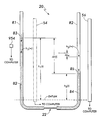
- FIG. 1 is a functional diagram of a test fluid flowing in an exemplary scanning tube viscometer (SCTV), e.g., a U-shaped tube having a capillary tube therein and with column level detectors and a single point detector monitoring the movement of the fluid;
- SCTV scanning tube viscometer
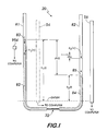
- FIG. 2 is a graphical representation of the height of the respective columns of fluid over time in the two legs of the U-shaped tube;
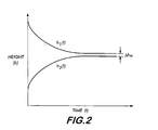
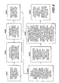
- FIG. 3 is a flowchart of the method of the present invention.
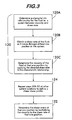
- FIG. 4 is a flowchart of the method of determining the fluid's characteristic viscosity-shear rate relationship
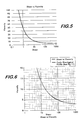
- FIG. 5 depicts a typical functional relationship between shear rate and viscosity
- FIG. 6 is a viscosity-shear rate curve with associated cyclic rheological profile
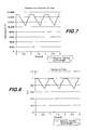
- FIG. 7 is a graphical depiction of the pressure in the artery as a function of time
- FIG. 8 is a graphical depiction of the flow rate in the artery, computed using a Windkessel model
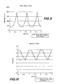
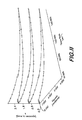
- FIG. 9 is a graphical depiction of the shear rate function
- FIG. 10 is a graphical depiction of the viscosity function
- FIG. 11 is a three-dimensional plot of the viscosity, shear rate and time.
- the method 120 (FIG. 3) of the present invention involves utilizing “scanning capillary tube viscometers” which are owned by the same Assignee of the present invention, namely, Rheologics, Inc. of Exton, Pa.
- scanning capillary tube viscometers are the subject matter of the following U.S. patents and patent applications:
- SCTVs scanning capillary tube viscometers
- the device monitors or detects the movement of the fluid under test as it experiences the plurality of shear rates and then from this movement, as well as using known dimensions of the passageways in the device, the viscosity of the fluid under test can be accurately and quickly determined.
- the diverted fluid remains unadulterated throughout the analysis.
- FIG. 1 is a functional diagram of the DRSC viscometer 20 which basically comprises a pair of riser tubes R 1 and R 2 and a capillary tube 22 coupled between them (although it should be understood that the position of the capillary tube 22 is not limited to the position shown, but as discussed in U.S. Pat. No.
- FIG. 2 is a graphical representation of the height of the respective columns of fluid over time.
- the DRSC viscometer 20 is used by way of example only and that any of the other SCTVs could be used and wherein the data collected from those SCTVs may include the changing weight, volume, etc., of the fluid moving through the SCTVs.
- the phrase “fluid movement data” used throughout this Specification is not limited to the changing heights of the fluid columns 82 / 84 and can represent any data about the fluid movement through any of these SCTVs. Where “height vs. time” data is mentioned, it is done by way of example only.
- V is the viscosity of the fluid under test
- S is the shear rate
- the coefficients f 1 , f 2 and f 3 are derived from both (i) parameters of the DRSC viscometer and (ii) data collected from the DRSC viscometer 20 when a portion of the fluid under test is run through the DRSC viscometer 20 . Once these coefficients are derived, the result is a viscosity-shear rate relationship or equation that describes the viscosity of that fluid in that system over all shear rates.
- the system is the circulatory system of a particular individual
- the result is a blood viscosity-shear relationship or equation unique to that individual.
- a physician can then determine a particular viscosity at any location in the cardiovascular system of that individual by simply detecting the shear rate of the blood at that location and then plugging the shear rate value into the relationship.
- the physician can now also determine the shear stress at that location by multiplying the viscosity of the fluid at that location with the shear rate at that location. Doing this at a plurality of locations, the physician can generate a shear stress profile of the entire cardiovascular system, a result heretofore unknown.
- equation 1 is by way of example only and that if a different SCTV were used, e.g., the Single Capillary Tube Viscometer of application Ser. No. 09/908,374, the form of equation (1) would be different; similarly, if a different constitutive equation model were used, e.g., Herschel-Bulkley model, instead of the Casson model, the form of equation (1) may also be different. However, the concept is the same: using the method 120 of the present invention yields a viscosity-shear rate relationship over all shear rates unique to that system.
- the method 120 of the present invention involves: determining a characteristic relationship for the fluid in a system between the viscosity an shear rate ( 120 A); obtaining a shear rate of the fluid as it moves through at least one position in the system ( 120 B); and determining the viscosity of the fluid at that one position as the fluid moves through that one position in the system by applying the shear rate to the characteristic relationship ( 120 C).
- the first step 120 A of determining the characteristic relationship will be discussed in detail later; suffice it to say that this relationship provides a viscosity-shear rate relationship for that particular fluid from approximately zero shear rate to infinite shear rate.
- the second step 120 B of obtaining a shear rate can be accomplished by any well-known method of detecting the shear rate of a fluid, e.g., using ultrasonic devices, Doppler devices, NMR devices, MRI devices, etc.
- the third step 120 C applies the detected shear rate to the characteristic equation from step 120 A to arrive at the particular viscosity for the fluid at the particular location where the shear rate was detected.
- This method 120 can be supplemented by determining the shear stress at that one position by multiplying the determined viscosity by the detected shear rate (step 122 ).
- a shear stress profile can be determined for the fluid flowing in the system (step 124 ).
- step 120 A involves determining the characteristic viscosity-shear rate relationship for the particular fluid.
- the following discussion describes the determination of equation 1, bearing in mind that the Casson model is used by way of example only and using the DRSC viscometer 20 , also by way of example only.
- the method of determining the fluid's characteristic viscosity-shear rate relationship includes the following steps:
- step1 Divert a portion of the fluid under test (FUT) into a Scanning Capillary Tube Viscometer (SCTV);
- step2 Use the SCTV to measure and record fluid movement data (e.g., fluid heights in the rising and falling tubes, changing weight, volume, etc.) at a sequence of equally spaced time points (observations of time);
- fluid movement data e.g., fluid heights in the rising and falling tubes, changing weight, volume, etc.
- step3 From the flow of data of step1, compute estimated values of the mean velocity of the FUT at the observation times;
- step4) Select a model for the constitutive equation that relates shear rate with shear stress.
- step 5 Using the constitutive equation and the general principles of fluid dynamics, determine a theoretical model which gives the mean flow velocity of the FUT as a function of time and other physical and constitutive equation parameters;
- step6 Substitute the fluid movement data of step2 into the equation of step5 to arrive at an overdetermined system of equations for the parameters of step5, one equation for each observation time.
- a typical equation expresses the theoretical value of the mean velocity corresponding to a single observation time in terms of the unknown parameter values;
- step 7 Apply a non-linear curve-fitting algorithm to determine the values of the parameters of step5 which minimize the sum of squares of the deviations of the theoretical values of the mean velocity of step5 and the corresponding estimated values of mean velocity from step3.
- the resulting set of parameter values provide a numerical description of the particular FUT, based on the particular SCTV device, constitutive equation, and curve-fitting technique;
- step8 Use the set of parameter values of step6 to determine an equation which allows determination of the viscosity of the FUT in terms of a given value for the shear rate.
- the DRSC viscometer 20 comprises two identical riser tubes connected by a capillary tube 22 of significantly smaller diameter.
- a falling column of fluid 82 is present in riser tube R 1 and a rising column of fluid 84 is present in the other riser tube R 2 .
- the shear rate and viscosity are estimated at the endpoints of the various time intervals. If S denotes the shear rate and V denotes the viscosity, then both are functions of time, as given by the following parametric equations:
- V V ( t )
- the viscosity is a decreasing function of the shear rate, so that, ideally, the parameter t may be eliminated and viscosity described as a function of shear rate:
- V F ( S )
- shear rate-viscosity algorithm it is the purpose of the shear rate-viscosity algorithm to compute the functional relationship between shear and viscosity as well as to compute additional parameters describing the fluid flow through the capillary tube 22 during the test period. As part of the algorithm, noise is filtered from the observed data.
- ⁇ the density of the fluid under test
- R c the radius of the capillary tube 22 ;
- L the length of the capillary tube 22 ;
- y(t) the mean flow velocity at the riser tubes R 1 /R 2 ;
- R r the (common) radius of the riser tubes R 1 /R 2 ;
- x 1 (t) the height of the falling tube in mm at time t
- x 2 (t) the height of the riser tube in mm at time t
- ⁇ y and a 3 are constants.
- the parameter ⁇ y is called the yield stress and will be discussed shortly.
- R c denote the radius of the capillary tube 22 .
- the shear stress ⁇ is a function of r (and t).
- the location at the wall of the capillary tube 22 the value of the shear stress is called the wall stress.
- the shear rate S can be expressed as a function S(y) of the velocity. Furthermore, the quantities a 1 ,a 2 ,a 3 are constant and, in particular, do not depend on t.
- the viscosity equation represents the viscosity-shear rate relationship for a fluid flowing through a system (e.g., blood in the body; hydraulic fluid in a control system, oil in engine system, etc.). Therefore, to find the viscosity (or shear stress) of that fluid at any point in the system, one need only detect the shear rate at that point and then plug the shear rate into the equation.
- equation 1 gives the value of the viscosity for any shear rate, it does not describe what shear rates are actually being attained within an actual artery or the relative durations of such viscosities. Thus, the following discussion addresses these issues.
- the variable t measures time within this cycle; ⁇ (t) denotes the viscosity in a specified artery at time t and ⁇ ave denotes the time average of ⁇ (t) over the cardiac cycle.
- the variable ⁇ (t) is known as the “cyclic rheological profile” and ⁇ ave is known as the “average cyclic viscosity” (ACV) of the artery.
- ACV average cyclic viscosity
- the equation (1) provides a relationship between shear rate S and viscosity V.
- This relationship may be plotted consisting of the points (S,V) for every possible shear rate S. (See FIG. 6.)
- the curve is subject-dependent and gives a complete rheological profile of the subject (that is, it gives the viscosity at at all shear rates).
- this rheological profile does not give any information about what viscosities are actually achieved in the subject's arteries and the proportion of time spent at each viscosity. That is precisely the information provided by the functions ⁇ (t) and ⁇ dot over ( ⁇ ) ⁇ (t).
- FIGS. 9 and 10 A model based on the classic Windkessel flow model is used lo compute the flow rate as a function of time. The result is given in FIG. 8 .
- the main result of methodology is to provide a technique to calculate the shear rate and viscosity as a function of time, as shown in FIGS. 9 and 10, respectively.
- FIG. 6 shows the portion of the shear-viscosity curve which is actually traversed by the blood flow: the cyclic Theological profile. This is just the graph of the pair of parametric equations:
- V ⁇ ( t )
- FIG. 11 shows a three-dimensional representation of the relationship between time, shear and viscosity. This graph shows not only which shear-viscosity pairs are traversed, but the time sequence of the traversal.
- the average cyclic rheological profile is given by:
- the viscosity ranges between 3.89 and 6.90.
- the time average of the viscosity values is 5.58.
- the technique for calculating the functions ⁇ dot over ( ⁇ ) ⁇ (t) and ⁇ (t) are referred to as the cyclic rheological profile algorithm which comprises two parts:
- the capillary tube 22 of the DRSC viscometer 20 may be used as the “virtual” artery and wherein R c represents the radius of the capillary tube 22 and R represents the radii of riser tubes R 1 /R 2 . Furthermore, as described in detail earlier, the DRSC viscometer 20 is used to calculate the associated curve-fitting constants a 1 ,a 2 ,a 3 corresponding to the flow of the blood through the viscometer 20 , as well as the constants c and c 1 (as defined earlier with respect to equation 2-21 and 2-23).
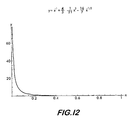
- y ⁇ ( t ) ca 2 a 3 ⁇ [ ( c 1 ⁇ ) - 1 + 4 3 - 1 21 ⁇ ⁇ ( c 1 ⁇ ) 3 - 16 7 ⁇ ⁇ ( c 1 ⁇ ) - 1 / 2 ]
- h ca 2 a 3 ⁇ [ w - 1 + 4 3 - 1 21 ⁇ ⁇ w 3 - 16 7 ⁇ ⁇ w - 1 / 2 ]
- ⁇ ⁇ ( t ) f 1 + f 2 ⁇ . ⁇ ( t ) + f 3 ⁇ . ⁇ ( t )
- ⁇ a (t) denotes the viscosity function of an actual artery at time t.
- the computation of ⁇ a (t) must address the following issues:
- An actual artery possibly has different geometry (radius and length) than the virtual artery.
- the flow rate y(t) through an actual artery is periodic with period equal to the length of a cardiac cycle, as opposed to the flow rate for the virtual artery, which is a decreasing function of t.
- the function ⁇ a (t) is a periodic function of t, with period equal to the length of a cardiac cycle, as opposed to the function ⁇ (t), which is a decreasing function of t.
- y y the velocity of blood in the artery at systole
- y d the velocity of blood in the artery at diastole
- R s the radius of the artery at systole
- R d the radius of the artery at diastole
- the pulse-pressure function iv. is determined using a measuring device under development by the Assignee, namely, Rheologics, Inc. Determination of the physical constants of iii will be discussed below.
- the DRSC viscometer 20 comprises a U-shaped device with two identical riser tubes connected by a capillary tube 22 of significantly smaller diameter.
- a “falling column of fluid 82 is generated and a rising column of fluid 84 is generated.
- the shear rate and viscosity are estimated at the endpoints of the various time intervals. Using ⁇ dot over ( ⁇ ) ⁇ to denote the shear rate and ⁇ the viscosity, then both are functions of time, and form parametric equations:
- g gravitational acceleration in meters/s 2 ;
- ⁇ the density of the fluid being tests in kg/m 3 ;
- R c the radius of the capillary tube in meters
- L the length of the capillary tube in meters
- y(t) the mean flow velocity at the riser tube in meters/second
- R r the (common) radius of the riser tubes in meters
- x 1 (t) the height of the falling tube in meters at time t;
- x 2 (t) the height of the riser tube in meters at time t;
- ⁇ y the yield stress in the capillary tube 22 .
- a 3 is a constant which depends only on the geometry of the DRSC viscometer 20 and not on t.
- P(t) denotes the blood pressure in an artery at time t and can be obtained using pulse pressure data collected by a pulse pressure device.
- the device may comprise an arm pressure cuff which auto inflates to a predetermined pressure setable in software (currently approx. 170 MM Hg). It then auto-deflates through a small orifice. After about a 1 second delay (also software setable), a pressure sensor and associated circuitry starts collecting pressure data at 400 samples per second for about 5 seconds. The data is stored in a random access memory module (RAM, e.g., Compact Flash). The cuff then rapidly deflates any remaining pressure.
- RAM random access memory module
- the data is now downloaded to a computer using a serial port and Windows hyper terminal and saved to a raw file. It is then imported into Excel and converted to appropriate numbers and graphed.
- the power supply is a 12V DC wall power pack
- P(t) is sampled at the same rate at the functions x 2 (t) and y(t), and is measured in compatible units to those functions.
- the pulse pressure function is denoted by P(t) and represents the blood pressure in an actual artery at time t.
- the function P(t) is periodic, with constant period T 0 , where T 0 corresponds to the length of a cardiac cycle.
- the Windkessel model which connects blood pressure with the flow rate through the artery, is selected.
- Equation (4-6) gives the values of C and R in terms of the parameters (4-2).
- the pressure function P(t) is known.
- T d can be determined by numerical differentiation from P(t).
- the value of T d may be determined by locating the value of t at which P(t) is minimized.
- the values of P s ,P d , ⁇ dot over (P) ⁇ s , ⁇ dot over (P) ⁇ d may then be determined.
- the derivative ⁇ dot over (P) ⁇ (t) may be calculated by differentiating P(t) numerically.
- T d may be determined as the time at which P(t) assumes its minimum value.
- y s ,y d ,P s ,P d , ⁇ dot over (P) ⁇ s , ⁇ dot over (P) ⁇ d may be computed.
- This constant depends on the physical properties of blood and the geometry of the measuring apparatus.
- CT(y) Since the function y is monotone for 0 ⁇ x ⁇ 1, then y has an inverse function, which is denoted CT(y), and defined by the property:
- CT(y) is called the Casson Transform corresponding to the parameter values a 2 ,a 3 .
- the Casson Transform is sometimes denoted as CT(y;a 2 ,a 3 ).
- CT(y) is defined as an inverse function
- CT(y) is defined for 0 ⁇ y ⁇ .
- CT(y) is monotone decreasing throughout its domain.
- CT(y) is concave up throughout its domain.
- CT(y) is has continuous first and second derivatives throughout its domain.
- CT(y) denotes the Casson Transform, whose value may be calculated using Theorem 5.1.
- a 1 ,a 2 ,a 3 be the curve-fitting parameters obtained from testing a sample using a capillary of radius R c .
- CT(y) denotes the Casson transform.
- the pulse-pressure function P(t) for the flow through the artery at times t in the interval 0 ⁇ t ⁇ T 0 , where T 0 is the length of a single cardiac cycle is assumed to be known. Also, from the function P(t), it was previously shown how to compute the function y(t) which gives the velocity of flow through the artery. In the following discussion, it is assumed that the radius of the artery remains fixed throughout the cardiac cycle. That is, the pulsation of the artery is ignored as a function of time. This will be addressed later.
- ⁇ ave 1 T 0 ⁇ ⁇ 0 T 0 ⁇ ⁇ ⁇ ( t ) ⁇ ⁇ t .
- ⁇ ave a 3 + 2 ⁇ a 3 T 0 ⁇ ⁇ 0 T 0 ⁇ ⁇ t ⁇ ⁇ ( k - 3 ⁇ y ⁇ ( t ) ) + a 3 T 0 ⁇ ⁇ 0 T 0 ⁇ ⁇ t ⁇ ⁇ ( k - 3 ⁇ y ⁇ ( t ) ) 2 ( 8 ⁇ - ⁇ 2 )
- y(t) is computed using Theorem 4.1.
- y ⁇ ( t ) y 0 + l ⁇ ⁇ ⁇ L ⁇ ⁇ 0 t ⁇ P ⁇ ( u ) ⁇ ⁇ u ⁇ ⁇ ( 0 ⁇ t ⁇ T 0 ) ( 8 ⁇ - ⁇ 4 )
- the function ⁇ depends on the elastic properties of the artery wall, varies from patient to patient, and even varies with time for a particular patient (due to exercise, stress, and arterial disease).
- V denote the value of the artery when its radius is R.
- the compliance function may vary with time (say due to arterial disease). However, for purposes of this analysis, it is assumed that an unchanging compliance function is present.
- the inequalities (9-4), (9-6), and (9-8) give requirements that any radius-pressure model must satisfy.
- inequality (9-4) is automatically satisfied. Furthermore, for inequality (9-6) to be satisfied, there must be:
- ⁇ R d R s ( 10 ⁇ - ⁇ 3 )
- ⁇ P d P s
- R d , R s denote the radius at diastole and systole, respectively, and P d , P s denote, respectively, the pressure at diastole and systole, respectively.
- CT(y) denotes the Casson transform.
- ⁇ ave a a 3 + 2 ⁇ a 3 T 0 ⁇ ⁇ 0 T 0 ⁇ ⁇ t ⁇ ⁇ ( k - 3 ⁇ y ⁇ ( t ) ) + a 3 T 0 ⁇ ⁇ 0 T 0 ⁇ ⁇ t ⁇ ⁇ ( k - 3 ⁇ y ⁇ ( t ) ) 2 ( 11 ⁇ - ⁇ 1 )
- the value of pressure is a maximum as is the radius.
- R s represents the maximum artery radius.
- R d represents the minimum value of the artery radius. Based on experiment, it is possible to determine an approximation for the ratio R d /R s and use this experimental ratio, independent of the subject. In the absence of such experimental values, it is assumed that this ratio is 0.5. That is, it is assumed that the artery contracts to half its radius from systole to diastole. Assuming that the ratio R d /R s is known, then the value of R d may be determined from the value of R s . For a more accurate approach, the value of R d may be determined using an MRI.
- the approach to determining the velocity values y s and y d can mimic the approach to determining R s and R d . Namely, average values can be assumed for a particular artery for a simple, subject-independent approach or a more elaborate approach can be used to obtain subject-dependent values. In all cases, using a subject-independent approach may be used for general screening, and a subject-dependent approach where arterial disease is present or suspected.
Abstract
Description


Claims (7)


Priority Applications (1)
| Application Number | Priority Date | Filing Date | Title |
|---|---|---|---|
| US10/245,237 US6796168B1 (en) | 2000-08-28 | 2002-09-17 | Method for determining a characteristic viscosity-shear rate relationship for a fluid |
Applications Claiming Priority (4)
| Application Number | Priority Date | Filing Date | Title |
|---|---|---|---|
| US22861200P | 2000-08-28 | 2000-08-28 | |
| US09/789,350 US20010039828A1 (en) | 1999-11-12 | 2001-02-21 | Mass detection capillary viscometer |
| US09/897,164 US6484565B2 (en) | 1999-11-12 | 2001-07-02 | Single riser/single capillary viscometer using mass detection or column height detection |
| US10/245,237 US6796168B1 (en) | 2000-08-28 | 2002-09-17 | Method for determining a characteristic viscosity-shear rate relationship for a fluid |
Related Parent Applications (1)
| Application Number | Title | Priority Date | Filing Date |
|---|---|---|---|
| US09/897,164 Continuation-In-Part US6484565B2 (en) | 1999-11-12 | 2001-07-02 | Single riser/single capillary viscometer using mass detection or column height detection |
Publications (1)
| Publication Number | Publication Date |
|---|---|
| US6796168B1 true US6796168B1 (en) | 2004-09-28 |
Family
ID=27397862
Family Applications (4)
| Application Number | Title | Priority Date | Filing Date |
|---|---|---|---|
| US09/897,164 Expired - Fee Related US6484565B2 (en) | 1999-11-12 | 2001-07-02 | Single riser/single capillary viscometer using mass detection or column height detection |
| US10/156,316 Expired - Fee Related US6523396B2 (en) | 1999-11-12 | 2002-05-28 | Single riser/single capillary viscometer using mass detection or column height detection |
| US10/156,165 Expired - Fee Related US6571608B2 (en) | 1999-11-12 | 2002-05-28 | Single riser/single capillary viscometer using mass detection or column height detection |
| US10/245,237 Expired - Lifetime US6796168B1 (en) | 2000-08-28 | 2002-09-17 | Method for determining a characteristic viscosity-shear rate relationship for a fluid |
Family Applications Before (3)
| Application Number | Title | Priority Date | Filing Date |
|---|---|---|---|
| US09/897,164 Expired - Fee Related US6484565B2 (en) | 1999-11-12 | 2001-07-02 | Single riser/single capillary viscometer using mass detection or column height detection |
| US10/156,316 Expired - Fee Related US6523396B2 (en) | 1999-11-12 | 2002-05-28 | Single riser/single capillary viscometer using mass detection or column height detection |
| US10/156,165 Expired - Fee Related US6571608B2 (en) | 1999-11-12 | 2002-05-28 | Single riser/single capillary viscometer using mass detection or column height detection |
Country Status (3)
| Country | Link |
|---|---|
| US (4) | US6484565B2 (en) |
| AU (1) | AU2001281219A1 (en) |
| WO (1) | WO2002018908A2 (en) |
Cited By (15)
| Publication number | Priority date | Publication date | Assignee | Title |
|---|---|---|---|---|
| US20050214131A1 (en) * | 2002-08-21 | 2005-09-29 | Medquest Products, Inc. | Methods and systems for determining a viscosity of a fluid |
| WO2008109185A2 (en) * | 2007-03-06 | 2008-09-12 | Kensey Kenneth R | A noninvasive method to determine characteristics of the heart |
| US20090090504A1 (en) * | 2007-10-05 | 2009-04-09 | Halliburton Energy Services, Inc. - Duncan | Determining Fluid Rheological Properties |
| US20090205410A1 (en) * | 2008-02-14 | 2009-08-20 | Meng-Yu Lin | Apparatus for measuring surface tension |
| US20100249620A1 (en) * | 2007-07-11 | 2010-09-30 | Cho Daniel J | Use of blood flow parameters to determine the propensity for atherothrombosis |
| US20110072890A1 (en) * | 2009-09-25 | 2011-03-31 | Bio-Visco Inc. | Device for automatically measuring viscosity of liquid |
| WO2011139282A1 (en) * | 2010-05-07 | 2011-11-10 | Rheovector Llc | Method for determining shear stress and viscosity distribution in a blood vessel |
| US20140105446A1 (en) * | 2012-10-12 | 2014-04-17 | Halliburton Energy Services, Inc. | Determining wellbore fluid properties |
| US9408541B2 (en) * | 2014-08-04 | 2016-08-09 | Yamil Kuri | System and method for determining arterial compliance and stiffness |
| US20160302672A1 (en) * | 2014-08-04 | 2016-10-20 | Yamil Kuri | System and Method for Determining Arterial Compliance and Stiffness |
| CN106053294A (en) * | 2016-06-18 | 2016-10-26 | 朱泽斌 | Double-capillary method and device for measuring liquid viscosity |
| US20160356689A1 (en) * | 2014-12-15 | 2016-12-08 | Halliburton Energy Services, Inc. | Yield stress measurement device and related methods |
| CN106896036A (en) * | 2017-01-13 | 2017-06-27 | 中国空间技术研究院 | A kind of embedding adhesive viscosity determining procedure |
| US20200348329A1 (en) * | 2019-05-01 | 2020-11-05 | Queen's University At Kingston | Apparatus and Method for Measuring Velocity Perturbations in a Fluid |
| US20230023301A1 (en) * | 2019-12-18 | 2023-01-26 | Tohoku University | Viscometer and method for measuring viscosity |
Families Citing this family (37)
| Publication number | Priority date | Publication date | Assignee | Title |
|---|---|---|---|---|
| JP3976953B2 (en) * | 1999-08-13 | 2007-09-19 | 森永乳業株式会社 | Method and apparatus for determining fluidity of fluid in container |
| US6484565B2 (en) | 1999-11-12 | 2002-11-26 | Drexel University | Single riser/single capillary viscometer using mass detection or column height detection |
| US20030158500A1 (en) * | 1999-11-12 | 2003-08-21 | Kenneth Kensey | Decreasing pressure differential viscometer |
| US6692437B2 (en) | 1999-11-12 | 2004-02-17 | Rheologics, Inc. | Method for determining the viscosity of an adulterated blood sample over plural shear rates |
| US6412336B2 (en) | 2000-03-29 | 2002-07-02 | Rheologics, Inc. | Single riser/single capillary blood viscometer using mass detection or column height detection |
| US8101209B2 (en) | 2001-10-09 | 2012-01-24 | Flamel Technologies | Microparticulate oral galenical form for the delayed and controlled release of pharmaceutical active principles |
| DE10236122A1 (en) * | 2002-08-07 | 2004-02-19 | Bayer Ag | Device and method for determining viscosities and liquids by means of capillary force |
| TWI323660B (en) | 2003-02-25 | 2010-04-21 | Otsuka Pharma Co Ltd | Pten inhibitor or maxi-k channels opener |
| US6997053B2 (en) * | 2003-08-27 | 2006-02-14 | The Boc Group, Inc. | Systems and methods for measurement of low liquid flow rates |
| US7013714B2 (en) * | 2003-09-30 | 2006-03-21 | Delphi Technologies, Inc. | Viscosity measurement apparatus |
| US20050169994A1 (en) * | 2003-11-25 | 2005-08-04 | Burke Matthew D. | Carvedilol free base, salts, anhydrous forms or solvates thereof, corresponding pharmaceutical compositions, controlled release formulations, and treatment or delivery methods |
| EP1691789B1 (en) * | 2003-11-25 | 2017-12-20 | SmithKline Beecham (Cork) Limited | Carvedilol free base, salts, anhydrous forms or solvate thereof, corresponding pharmaceutical compositions, controlled release formulations, and treatment or delivery methods |
| US7905095B2 (en) * | 2004-07-16 | 2011-03-15 | Spx Corporation | System for refrigerant charging with constant volume tank |
| CA2574086A1 (en) * | 2004-07-21 | 2006-02-23 | Medtronic, Inc. | Medical devices and methods for reducing localized fibrosis |
| EP1773993A2 (en) * | 2004-07-21 | 2007-04-18 | Medtronic, Inc. | METHODS FOR REDUCING OR PREVENTING LOCALIZED FIBROSIS USING SiRNA |
| US7188515B2 (en) * | 2004-09-24 | 2007-03-13 | The Regents Of The University Of Michigan | Nanoliter viscometer for analyzing blood plasma and other liquid samples |
| WO2007002572A2 (en) * | 2005-06-24 | 2007-01-04 | N-Zymeceuticals, Inc. | Nattokinase for reducing whole blood viscosity |
| US7730769B1 (en) | 2006-05-24 | 2010-06-08 | Kwon Kyung C | Capillary viscometers for use with Newtonian and non-Newtonian fluids |
| CN1877291B (en) * | 2006-07-10 | 2010-08-25 | 哈尔滨工业大学 | Apparatus for detecting filling performance of newly-mixed concrete |
| US20080127717A1 (en) * | 2006-11-30 | 2008-06-05 | Chevron Oronite S.A. | Alternative pressure viscometer device |
| US7752895B2 (en) * | 2006-11-30 | 2010-07-13 | Chevron Oronite S.A. | Method for using an alternate pressure viscometer |
| MX2009012583A (en) * | 2007-05-22 | 2010-03-08 | Otsuka Pharma Co Ltd | A medicament comprising a carbostyril derivative and donepezil for treating alzheimer's disease. |
| CN101118233B (en) * | 2007-08-31 | 2010-11-24 | 武汉理工大学 | Method for testing homogeneity of light aggregate concrete |
| US8037894B1 (en) | 2007-12-27 | 2011-10-18 | Intermolecular, Inc. | Maintaining flow rate of a fluid |
| US8220502B1 (en) | 2007-12-28 | 2012-07-17 | Intermolecular, Inc. | Measuring volume of a liquid dispensed into a vessel |
| CN101685059B (en) * | 2009-05-15 | 2011-05-04 | 河海大学 | Method for dynamically detecting rheological property of concrete on construction site |
| GB201016992D0 (en) * | 2010-10-08 | 2010-11-24 | Paraytec Ltd | Viscosity measurement apparatus and method |
| US8661878B2 (en) * | 2011-01-18 | 2014-03-04 | Spectro, Inc. | Kinematic viscometer and method |
| US8677807B2 (en) | 2011-07-18 | 2014-03-25 | Korea Institute Of Industrial Technology | Micro viscometer |
| US8667831B2 (en) | 2011-07-18 | 2014-03-11 | Korea Institute Of Industrial Technology | Micro viscometer |
| US8544316B2 (en) | 2011-07-18 | 2013-10-01 | Korea Institute Of Industrial Technology | Micro viscometer |
| CN102607996B (en) * | 2012-02-23 | 2013-10-23 | 哈尔滨工业大学 | Fresh concrete fluidity, viscosity, and filling property measuring apparatus |
| US9128022B2 (en) | 2012-05-18 | 2015-09-08 | Korea Institute Of Industrial Technology | Micro viscometers and methods of manufacturing the same |
| US20140232853A1 (en) | 2013-02-21 | 2014-08-21 | Neil E. Lewis | Imaging microviscometer |
| CN105573279B (en) * | 2015-12-31 | 2018-12-21 | 广州中国科学院先进技术研究所 | A method of industrial processes are monitored based on sensing data |
| CN107063929B (en) * | 2017-06-20 | 2023-08-25 | 广东海洋大学 | Device and method for rapidly measuring molecular weight of chitosan |
| CN111595728B (en) * | 2020-05-28 | 2021-10-08 | 中交一公局集团有限公司 | Inspection mold, vibration inspection device and asphalt mixture fluidity detection method |
Citations (83)
| Publication number | Priority date | Publication date | Assignee | Title |
|---|---|---|---|---|
| US1810992A (en) | 1926-01-07 | 1931-06-23 | Dallwitz-Wegner Richard Von | Method and means for determining the viscosity of liquid substances |
| US2343061A (en) | 1943-10-29 | 1944-02-29 | Irany Ernest Paul | Capillary viscometer |
| US2696734A (en) | 1950-05-03 | 1954-12-14 | Standard Oil Co | Viscometer for semifluid substances |
| US2700891A (en) | 1953-12-01 | 1955-02-01 | Montgomery R Shafer | Direct reading viscometer |
| US2934944A (en) | 1955-02-14 | 1960-05-03 | Gerber Prod | Continuous viscosimeter |
| US3071961A (en) | 1959-12-22 | 1963-01-08 | Exxon Research Engineering Co | Automatic viscometer and process of using same |
| US3116630A (en) | 1960-07-21 | 1964-01-07 | Sinclair Research Inc | Continuous viscosimeter |
| US3137161A (en) | 1959-10-01 | 1964-06-16 | Standard Oil Co | Kinematic viscosimeter |
| US3138950A (en) | 1961-03-20 | 1964-06-30 | Phillips Petroleum Co | Apparatus for concurrent measurement of polymer melt viscosities at high and low shear rates |
| US3277694A (en) | 1965-08-20 | 1966-10-11 | Cannon Instr Company | Viscometer |
| US3286511A (en) | 1963-01-17 | 1966-11-22 | Coulter Electronics | Viscosity measurement |
| US3342063A (en) | 1965-02-23 | 1967-09-19 | Technicon Instr | Blood-viscosity measuring apparatus |
| US3435665A (en) | 1966-05-20 | 1969-04-01 | Dow Chemical Co | Capillary viscometer |
| US3520179A (en) | 1968-06-19 | 1970-07-14 | John C Reed | Variable head rheometer for measuring non-newtonian fluids |
| US3604247A (en) | 1968-07-19 | 1971-09-14 | Anvar | Automatic viscosity meter |
| US3666999A (en) | 1970-06-22 | 1972-05-30 | Texaco Inc | Apparatus for providing signals corresponding to the viscosity of a liquid |
| US3680362A (en) | 1970-03-17 | 1972-08-01 | Kunstharsfabriek Synthese Nv | Viscosimeter |
| US3699804A (en) | 1970-01-22 | 1972-10-24 | Ciba Geigy Ag | Capillary viscometer |
| US3713328A (en) | 1971-02-24 | 1973-01-30 | Idemitsu Kosan Co | Automatic measurement of viscosity |
| US3720097A (en) | 1971-01-21 | 1973-03-13 | Univ Pennsylvania | Apparatus and method for measuring mammalian blood viscosity |
| US3782173A (en) | 1971-06-03 | 1974-01-01 | Akzo Nv | Viscosimeter |
| US3839901A (en) | 1972-11-17 | 1974-10-08 | E Finkle | Method and apparatus for measuring viscosity |
| US3908411A (en) | 1973-06-06 | 1975-09-30 | Michael E Fahmie | Unitized washing machine bushing |
| US3911728A (en) | 1973-02-19 | 1975-10-14 | Daillet S A Ets | Coagulation detection apparatus |
| US3952577A (en) | 1974-03-22 | 1976-04-27 | Canadian Patents And Development Limited | Apparatus for measuring the flow rate and/or viscous characteristics of fluids |
| US3967934A (en) | 1969-06-13 | 1976-07-06 | Baxter Laboratories, Inc. | Prothrombin timer |
| US3990295A (en) | 1974-09-16 | 1976-11-09 | Boehringer Ingelheim Gmbh | Apparatus and method for the performance of capillary viscosimetric measurements on non-homogeneous liquids |
| US3999538A (en) | 1975-05-22 | 1976-12-28 | Buren Philpot V Jun | Method of blood viscosity determination |
| US4149405A (en) | 1977-01-10 | 1979-04-17 | Battelle, Centre De Recherche De Geneve | Process for measuring the viscosity of a fluid substance |
| US4165632A (en) | 1976-03-27 | 1979-08-28 | Torsten Kreisel | Method of measuring the fluidity of liquids for medical and pharmaceutical purposes, and apparatus for performing the method |
| US4193293A (en) | 1977-04-28 | 1980-03-18 | E.L.V.I. S.P.A. | Apparatus for determining blood elasticity parameters |
| US4207870A (en) | 1978-06-15 | 1980-06-17 | Becton, Dickinson And Company | Blood sampling assembly having porous vent means vein entry indicator |
| US4302965A (en) | 1979-06-29 | 1981-12-01 | Phillips Petroleum Company | Viscometer |
| US4341111A (en) | 1979-03-05 | 1982-07-27 | Fresenius Ag | Process and apparatus for determining the visco elastic characteristics of fluids |
| FR2510257A1 (en) | 1981-07-21 | 1983-01-28 | Centre Nat Rech Scient | Rheometer for medicine or industry - has calibrated tube filled, emptied and rinsed according to signals from liq. level detectors |
| DE3138514A1 (en) | 1981-09-28 | 1983-04-14 | Klaus Dipl.-Ing. 5100 Aachen Mussler | Method and device for determining the flow behaviour of biological liquids |
| US4417584A (en) | 1981-05-25 | 1983-11-29 | Institut National De La Sante Et De La Recherche Medicale | Real-time measuring method and apparatus displaying flow velocities in a segment of vessel |
| US4426878A (en) | 1981-10-13 | 1984-01-24 | Core Laboratories, Inc. | Viscosimeter |
| US4432761A (en) | 1981-06-22 | 1984-02-21 | Abbott Laboratories | Volumetric drop detector |
| US4461830A (en) | 1983-01-20 | 1984-07-24 | Buren Philpot V Jun | Serum fibrinogen viscosity in clinical medicine |
| US4517830A (en) | 1982-12-20 | 1985-05-21 | Gunn Damon M | Blood viscosity instrument |
| US4519239A (en) | 1982-05-13 | 1985-05-28 | Holger Kiesewetter | Apparatus for determining the flow shear stress of suspensions in particular blood |
| US4554821A (en) | 1982-08-13 | 1985-11-26 | Holger Kiesewetter | Apparatus for determining the viscosity of fluids, in particular blood plasma |
| USH93H (en) | 1985-09-23 | 1986-07-01 | The United States Of America As Represented By The Secretary Of The Army | Elongational rheometer |
| US4616503A (en) | 1985-03-22 | 1986-10-14 | Analysts, Inc. | Timer trigger for capillary tube viscometer and method of measuring oil properties |
| US4637250A (en) | 1985-01-25 | 1987-01-20 | State University Of New York | Apparatus and method for viscosity measurements for Newtonian and non-Newtonian fluids |
| US4680958A (en) | 1985-07-18 | 1987-07-21 | Solvay & Cie | Apparatus for fast determination of the rheological properties of thermoplastics |
| US4680957A (en) | 1985-05-02 | 1987-07-21 | The Davey Company | Non-invasive, in-line consistency measurement of a non-newtonian fluid |
| US4750351A (en) | 1987-08-07 | 1988-06-14 | The United States Of America As Represented By The Secretary Of The Army | In-line viscometer |
| US4856322A (en) | 1988-02-17 | 1989-08-15 | Willett International Limited | Method and device for measuring the viscosity of an ink |
| US4858127A (en) | 1986-05-30 | 1989-08-15 | Kdl Technologies, Inc. | Apparatus and method for measuring native mammalian blood viscosity |
| US4884577A (en) | 1984-10-31 | 1989-12-05 | Merrill Edward Wilson | Process and apparatus for measuring blood viscosity directly and rapidly |
| US4899575A (en) | 1988-07-29 | 1990-02-13 | Research Foundation Of State University Of New York | Method and apparatus for determining viscosity |
| US4947678A (en) | 1988-03-07 | 1990-08-14 | Snow Brand Milk Products Co., Ltd. | Method for measurement of viscosity change in blood or the like and sensor thereof |
| US5099698A (en) | 1989-04-14 | 1992-03-31 | Merck & Co. | Electronic readout for a rotameter flow gauge |
| WO1992015878A1 (en) | 1991-03-04 | 1992-09-17 | Kensey Nash Corporation | Apparatus and method for determining deformability of red blood cells of a living being |
| US5222497A (en) | 1991-01-25 | 1993-06-29 | Nissho Corporation | Hollow needle for use in measurement of viscosity of liquid |
| US5224375A (en) | 1991-05-07 | 1993-07-06 | Skc Limited | Apparatus for automatically measuring the viscosity of a liquid |
| US5257529A (en) | 1990-12-28 | 1993-11-02 | Nissho Corporation | Method and device for measurement of viscosity of liquids |
| US5271398A (en) | 1991-10-09 | 1993-12-21 | Optex Biomedical, Inc. | Intra-vessel measurement of blood parameters |
| US5272912A (en) | 1992-03-30 | 1993-12-28 | Yayoi Co., Ltd. | Apparatus and method for measuring viscosities of liquids |
| US5327778A (en) | 1992-02-10 | 1994-07-12 | Park Noh A | Apparatus and method for viscosity measurements using a controlled needle viscometer |
| US5333497A (en) | 1991-11-05 | 1994-08-02 | Metron As | Method and apparatus for continuous measurement of liquid flow velocity |
| WO1994020832A1 (en) | 1993-03-03 | 1994-09-15 | Vianova Kunstharz Aktiengesellschaft | Process and device for finding the rheological properties of liquids |
| US5365776A (en) | 1992-07-06 | 1994-11-22 | Schott Gerate Gmbh | Process and device for determining the viscosity of liquids |
| EP0654286A1 (en) | 1993-06-04 | 1995-05-24 | Electromecanica Bekal, S.L. | Method for treating viral diseases |
| US5421328A (en) | 1992-06-29 | 1995-06-06 | Minnesota Mining And Manufacturing Company | Intravascular blood parameter sensing system |
| US5447440A (en) | 1993-10-28 | 1995-09-05 | I-Stat Corporation | Apparatus for assaying viscosity changes in fluid samples and method of conducting same |
| US5491408A (en) | 1990-07-20 | 1996-02-13 | Serbio | Device for detecting the change of viscosity of a liquid electrolyte by depolarization effect |
| US5494639A (en) | 1993-01-13 | 1996-02-27 | Behringwerke Aktiengesellschaft | Biosensor for measuring changes in viscosity and/or density of a fluid |
| US5629209A (en) | 1995-10-19 | 1997-05-13 | Braun, Sr.; Walter J. | Method and apparatus for detecting viscosity changes in fluids |
| US5686659A (en) | 1993-08-31 | 1997-11-11 | Boehringer Mannheim Corporation | Fluid dose flow and coagulation sensor for medical instrument |
| US5725563A (en) | 1993-04-21 | 1998-03-10 | Klotz; Antoine | Electronic device and method for adrenergically stimulating the sympathetic system with respect to the venous media |
| US5792660A (en) | 1996-10-02 | 1998-08-11 | University Of Medicine And Dentistry Of New Jersey | Comparative determinants of viscosity in body fluids obtained with probes providing increased sensitivity |
| WO1999010724A2 (en) | 1997-08-28 | 1999-03-04 | Visco Technologies, Inc. | Viscosity measuring apparatus and method of use |
| US6322524B1 (en) | 1997-08-28 | 2001-11-27 | Visco Technologies, Inc. | Dual riser/single capillary viscometer |
| US6322525B1 (en) | 1997-08-28 | 2001-11-27 | Visco Technologies, Inc. | Method of analyzing data from a circulating blood viscometer for determining absolute and effective blood viscosity |
| US6402703B1 (en) | 1997-08-28 | 2002-06-11 | Visco Technologies, Inc. | Dual riser/single capillary viscometer |
| US6412336B2 (en) | 2000-03-29 | 2002-07-02 | Rheologics, Inc. | Single riser/single capillary blood viscometer using mass detection or column height detection |
| US6428488B1 (en) | 1997-08-28 | 2002-08-06 | Kenneth Kensey | Dual riser/dual capillary viscometer for newtonian and non-newtonian fluids |
| US6450974B1 (en) | 1997-08-28 | 2002-09-17 | Rheologics, Inc. | Method of isolating surface tension and yield stress in viscosity measurements |
| US6484565B2 (en) | 1999-11-12 | 2002-11-26 | Drexel University | Single riser/single capillary viscometer using mass detection or column height detection |
| US6484566B1 (en) | 2000-05-18 | 2002-11-26 | Rheologics, Inc. | Electrorheological and magnetorheological fluid scanning rheometer |
Family Cites Families (13)
| Publication number | Priority date | Publication date | Assignee | Title |
|---|---|---|---|---|
| CH229225A (en) * | 1940-09-05 | 1943-10-15 | Inst Kunststoffe Und Anstrichf | Device for measuring the consistency of paints and varnishes. |
| FR1446894A (en) * | 1965-09-13 | 1966-07-22 | Continuous indicator and automatic regulator of the viscosity of a liquid | |
| CH540487A (en) | 1972-04-10 | 1973-08-15 | Ciba Geigy Ag | Capillary viscometer |
| FR2188146B1 (en) | 1972-06-02 | 1976-08-06 | Instr Con Analyse | |
| US3853121A (en) | 1973-03-07 | 1974-12-10 | B Mizrachy | Methods for reducing the risk of incurring venous thrombosis |
| US4495798A (en) * | 1982-12-12 | 1985-01-29 | Chesebrough-Pond's Inc. | Method and apparatus for measuring consistency of non-Newtonian fluids |
| GB8302938D0 (en) * | 1983-02-03 | 1983-03-09 | Cooper A A | Viscosity control |
| DE3331659C2 (en) * | 1983-09-02 | 1986-07-24 | Bayer Ag, 5090 Leverkusen | Device for measuring viscosity |
| FR2572527B1 (en) | 1984-10-30 | 1987-12-11 | Bertin & Cie | METHOD AND DEVICE FOR MEASURING RHEOLOGICAL CHARACTERISTICS OF A FLUID, PARTICULARLY A BIOLOGICAL FLUID SUCH AS BLOOD |
| FR2664982B1 (en) | 1990-07-20 | 1994-04-29 | Serbio | APPARATUS FOR DETECTING CHANGE IN VISCOSITY, BY MEASURING RELATIVE SLIDING, PARTICULARLY FOR DETECTING BLOOD COAGULATION TIME. |
| JPH0827229B2 (en) * | 1990-12-28 | 1996-03-21 | 株式会社ニッショー | Liquid viscosity measuring method and apparatus |
| US5443078A (en) | 1992-09-14 | 1995-08-22 | Interventional Technologies, Inc. | Method for advancing a guide wire |
| DE19809530C1 (en) * | 1998-03-05 | 1999-07-29 | Joachim Laempe | Method and apparatus for measuring and/or controlling the homogenization state of a suspension |
-
2001
- 2001-07-02 US US09/897,164 patent/US6484565B2/en not_active Expired - Fee Related
- 2001-08-09 WO PCT/US2001/025007 patent/WO2002018908A2/en active Search and Examination
- 2001-08-09 AU AU2001281219A patent/AU2001281219A1/en not_active Abandoned
-
2002
- 2002-05-28 US US10/156,316 patent/US6523396B2/en not_active Expired - Fee Related
- 2002-05-28 US US10/156,165 patent/US6571608B2/en not_active Expired - Fee Related
- 2002-09-17 US US10/245,237 patent/US6796168B1/en not_active Expired - Lifetime
Patent Citations (92)
| Publication number | Priority date | Publication date | Assignee | Title |
|---|---|---|---|---|
| US1810992A (en) | 1926-01-07 | 1931-06-23 | Dallwitz-Wegner Richard Von | Method and means for determining the viscosity of liquid substances |
| US2343061A (en) | 1943-10-29 | 1944-02-29 | Irany Ernest Paul | Capillary viscometer |
| US2696734A (en) | 1950-05-03 | 1954-12-14 | Standard Oil Co | Viscometer for semifluid substances |
| US2700891A (en) | 1953-12-01 | 1955-02-01 | Montgomery R Shafer | Direct reading viscometer |
| US2934944A (en) | 1955-02-14 | 1960-05-03 | Gerber Prod | Continuous viscosimeter |
| US3137161A (en) | 1959-10-01 | 1964-06-16 | Standard Oil Co | Kinematic viscosimeter |
| US3071961A (en) | 1959-12-22 | 1963-01-08 | Exxon Research Engineering Co | Automatic viscometer and process of using same |
| US3116630A (en) | 1960-07-21 | 1964-01-07 | Sinclair Research Inc | Continuous viscosimeter |
| US3138950A (en) | 1961-03-20 | 1964-06-30 | Phillips Petroleum Co | Apparatus for concurrent measurement of polymer melt viscosities at high and low shear rates |
| US3286511A (en) | 1963-01-17 | 1966-11-22 | Coulter Electronics | Viscosity measurement |
| US3342063A (en) | 1965-02-23 | 1967-09-19 | Technicon Instr | Blood-viscosity measuring apparatus |
| US3277694A (en) | 1965-08-20 | 1966-10-11 | Cannon Instr Company | Viscometer |
| US3435665A (en) | 1966-05-20 | 1969-04-01 | Dow Chemical Co | Capillary viscometer |
| US3520179A (en) | 1968-06-19 | 1970-07-14 | John C Reed | Variable head rheometer for measuring non-newtonian fluids |
| US3604247A (en) | 1968-07-19 | 1971-09-14 | Anvar | Automatic viscosity meter |
| US3967934A (en) | 1969-06-13 | 1976-07-06 | Baxter Laboratories, Inc. | Prothrombin timer |
| US3699804A (en) | 1970-01-22 | 1972-10-24 | Ciba Geigy Ag | Capillary viscometer |
| US3680362A (en) | 1970-03-17 | 1972-08-01 | Kunstharsfabriek Synthese Nv | Viscosimeter |
| US3666999A (en) | 1970-06-22 | 1972-05-30 | Texaco Inc | Apparatus for providing signals corresponding to the viscosity of a liquid |
| US3720097A (en) | 1971-01-21 | 1973-03-13 | Univ Pennsylvania | Apparatus and method for measuring mammalian blood viscosity |
| US3713328A (en) | 1971-02-24 | 1973-01-30 | Idemitsu Kosan Co | Automatic measurement of viscosity |
| US3782173A (en) | 1971-06-03 | 1974-01-01 | Akzo Nv | Viscosimeter |
| US3839901A (en) | 1972-11-17 | 1974-10-08 | E Finkle | Method and apparatus for measuring viscosity |
| US3911728A (en) | 1973-02-19 | 1975-10-14 | Daillet S A Ets | Coagulation detection apparatus |
| US3908411A (en) | 1973-06-06 | 1975-09-30 | Michael E Fahmie | Unitized washing machine bushing |
| US3952577A (en) | 1974-03-22 | 1976-04-27 | Canadian Patents And Development Limited | Apparatus for measuring the flow rate and/or viscous characteristics of fluids |
| US3990295A (en) | 1974-09-16 | 1976-11-09 | Boehringer Ingelheim Gmbh | Apparatus and method for the performance of capillary viscosimetric measurements on non-homogeneous liquids |
| US3999538A (en) | 1975-05-22 | 1976-12-28 | Buren Philpot V Jun | Method of blood viscosity determination |
| US4083363A (en) | 1975-05-22 | 1978-04-11 | Buren Philpot V Jun | Blood viscosity determination device |
| US3999538B1 (en) | 1975-05-22 | 1984-07-24 | ||
| US4165632A (en) | 1976-03-27 | 1979-08-28 | Torsten Kreisel | Method of measuring the fluidity of liquids for medical and pharmaceutical purposes, and apparatus for performing the method |
| US4149405A (en) | 1977-01-10 | 1979-04-17 | Battelle, Centre De Recherche De Geneve | Process for measuring the viscosity of a fluid substance |
| US4193293A (en) | 1977-04-28 | 1980-03-18 | E.L.V.I. S.P.A. | Apparatus for determining blood elasticity parameters |
| US4207870A (en) | 1978-06-15 | 1980-06-17 | Becton, Dickinson And Company | Blood sampling assembly having porous vent means vein entry indicator |
| US4341111A (en) | 1979-03-05 | 1982-07-27 | Fresenius Ag | Process and apparatus for determining the visco elastic characteristics of fluids |
| US4302965A (en) | 1979-06-29 | 1981-12-01 | Phillips Petroleum Company | Viscometer |
| US4417584A (en) | 1981-05-25 | 1983-11-29 | Institut National De La Sante Et De La Recherche Medicale | Real-time measuring method and apparatus displaying flow velocities in a segment of vessel |
| US4432761A (en) | 1981-06-22 | 1984-02-21 | Abbott Laboratories | Volumetric drop detector |
| FR2510257A1 (en) | 1981-07-21 | 1983-01-28 | Centre Nat Rech Scient | Rheometer for medicine or industry - has calibrated tube filled, emptied and rinsed according to signals from liq. level detectors |
| DE3138514A1 (en) | 1981-09-28 | 1983-04-14 | Klaus Dipl.-Ing. 5100 Aachen Mussler | Method and device for determining the flow behaviour of biological liquids |
| US4426878A (en) | 1981-10-13 | 1984-01-24 | Core Laboratories, Inc. | Viscosimeter |
| US4519239A (en) | 1982-05-13 | 1985-05-28 | Holger Kiesewetter | Apparatus for determining the flow shear stress of suspensions in particular blood |
| US4554821A (en) | 1982-08-13 | 1985-11-26 | Holger Kiesewetter | Apparatus for determining the viscosity of fluids, in particular blood plasma |
| US4517830A (en) | 1982-12-20 | 1985-05-21 | Gunn Damon M | Blood viscosity instrument |
| US4461830A (en) | 1983-01-20 | 1984-07-24 | Buren Philpot V Jun | Serum fibrinogen viscosity in clinical medicine |
| US4884577A (en) | 1984-10-31 | 1989-12-05 | Merrill Edward Wilson | Process and apparatus for measuring blood viscosity directly and rapidly |
| US4637250A (en) | 1985-01-25 | 1987-01-20 | State University Of New York | Apparatus and method for viscosity measurements for Newtonian and non-Newtonian fluids |
| US4616503A (en) | 1985-03-22 | 1986-10-14 | Analysts, Inc. | Timer trigger for capillary tube viscometer and method of measuring oil properties |
| US4680957A (en) | 1985-05-02 | 1987-07-21 | The Davey Company | Non-invasive, in-line consistency measurement of a non-newtonian fluid |
| US4680958A (en) | 1985-07-18 | 1987-07-21 | Solvay & Cie | Apparatus for fast determination of the rheological properties of thermoplastics |
| USH93H (en) | 1985-09-23 | 1986-07-01 | The United States Of America As Represented By The Secretary Of The Army | Elongational rheometer |
| US4858127A (en) | 1986-05-30 | 1989-08-15 | Kdl Technologies, Inc. | Apparatus and method for measuring native mammalian blood viscosity |
| US4750351A (en) | 1987-08-07 | 1988-06-14 | The United States Of America As Represented By The Secretary Of The Army | In-line viscometer |
| US4856322A (en) | 1988-02-17 | 1989-08-15 | Willett International Limited | Method and device for measuring the viscosity of an ink |
| US4947678A (en) | 1988-03-07 | 1990-08-14 | Snow Brand Milk Products Co., Ltd. | Method for measurement of viscosity change in blood or the like and sensor thereof |
| US4899575A (en) | 1988-07-29 | 1990-02-13 | Research Foundation Of State University Of New York | Method and apparatus for determining viscosity |
| US5099698A (en) | 1989-04-14 | 1992-03-31 | Merck & Co. | Electronic readout for a rotameter flow gauge |
| US5491408A (en) | 1990-07-20 | 1996-02-13 | Serbio | Device for detecting the change of viscosity of a liquid electrolyte by depolarization effect |
| US5257529A (en) | 1990-12-28 | 1993-11-02 | Nissho Corporation | Method and device for measurement of viscosity of liquids |
| US5222497A (en) | 1991-01-25 | 1993-06-29 | Nissho Corporation | Hollow needle for use in measurement of viscosity of liquid |
| WO1992015878A1 (en) | 1991-03-04 | 1992-09-17 | Kensey Nash Corporation | Apparatus and method for determining deformability of red blood cells of a living being |
| US5224375A (en) | 1991-05-07 | 1993-07-06 | Skc Limited | Apparatus for automatically measuring the viscosity of a liquid |
| US5271398A (en) | 1991-10-09 | 1993-12-21 | Optex Biomedical, Inc. | Intra-vessel measurement of blood parameters |
| US5333497A (en) | 1991-11-05 | 1994-08-02 | Metron As | Method and apparatus for continuous measurement of liquid flow velocity |
| US5327778A (en) | 1992-02-10 | 1994-07-12 | Park Noh A | Apparatus and method for viscosity measurements using a controlled needle viscometer |
| US5272912A (en) | 1992-03-30 | 1993-12-28 | Yayoi Co., Ltd. | Apparatus and method for measuring viscosities of liquids |
| US5421328A (en) | 1992-06-29 | 1995-06-06 | Minnesota Mining And Manufacturing Company | Intravascular blood parameter sensing system |
| US5365776A (en) | 1992-07-06 | 1994-11-22 | Schott Gerate Gmbh | Process and device for determining the viscosity of liquids |
| US5494639A (en) | 1993-01-13 | 1996-02-27 | Behringwerke Aktiengesellschaft | Biosensor for measuring changes in viscosity and/or density of a fluid |
| WO1994020832A1 (en) | 1993-03-03 | 1994-09-15 | Vianova Kunstharz Aktiengesellschaft | Process and device for finding the rheological properties of liquids |
| US5725563A (en) | 1993-04-21 | 1998-03-10 | Klotz; Antoine | Electronic device and method for adrenergically stimulating the sympathetic system with respect to the venous media |
| EP0654286A1 (en) | 1993-06-04 | 1995-05-24 | Electromecanica Bekal, S.L. | Method for treating viral diseases |
| US5686659A (en) | 1993-08-31 | 1997-11-11 | Boehringer Mannheim Corporation | Fluid dose flow and coagulation sensor for medical instrument |
| US5447440A (en) | 1993-10-28 | 1995-09-05 | I-Stat Corporation | Apparatus for assaying viscosity changes in fluid samples and method of conducting same |
| US5629209A (en) | 1995-10-19 | 1997-05-13 | Braun, Sr.; Walter J. | Method and apparatus for detecting viscosity changes in fluids |
| US5792660A (en) | 1996-10-02 | 1998-08-11 | University Of Medicine And Dentistry Of New Jersey | Comparative determinants of viscosity in body fluids obtained with probes providing increased sensitivity |
| WO1999010724A2 (en) | 1997-08-28 | 1999-03-04 | Visco Technologies, Inc. | Viscosity measuring apparatus and method of use |
| US6322524B1 (en) | 1997-08-28 | 2001-11-27 | Visco Technologies, Inc. | Dual riser/single capillary viscometer |
| US6077234A (en) | 1997-08-28 | 2000-06-20 | Visco Technologies, Inc. | In-vivo apparatus and method of use for determining the effects of materials, conditions, activities, and lifestyles on blood parameters |
| US6152888A (en) | 1997-08-28 | 2000-11-28 | Visco Technologies, Inc. | Viscosity measuring apparatus and method of use |
| US6193667B1 (en) | 1997-08-28 | 2001-02-27 | Visco Technologies, Inc. | Methods of determining the effect(s) of materials, conditions, activities and lifestyles |
| US6200277B1 (en) | 1997-08-28 | 2001-03-13 | Visco Technologies, Inc. | In-vivo apparatus and methods of use for determining the effects of materials, conditions, activities, and lifestyles on blood parameters |
| US6261244B1 (en) | 1997-08-28 | 2001-07-17 | Visco Technologies, Inc. | Viscosity measuring apparatus and method of use |
| US6019735A (en) | 1997-08-28 | 2000-02-01 | Visco Technologies, Inc. | Viscosity measuring apparatus and method of use |
| US6322525B1 (en) | 1997-08-28 | 2001-11-27 | Visco Technologies, Inc. | Method of analyzing data from a circulating blood viscometer for determining absolute and effective blood viscosity |
| US6402703B1 (en) | 1997-08-28 | 2002-06-11 | Visco Technologies, Inc. | Dual riser/single capillary viscometer |
| US6450974B1 (en) | 1997-08-28 | 2002-09-17 | Rheologics, Inc. | Method of isolating surface tension and yield stress in viscosity measurements |
| US6428488B1 (en) | 1997-08-28 | 2002-08-06 | Kenneth Kensey | Dual riser/dual capillary viscometer for newtonian and non-newtonian fluids |
| US6443911B1 (en) | 1997-08-28 | 2002-09-03 | Visco Technologies, Inc. | Viscosity measuring apparatus and method of use |
| US6484565B2 (en) | 1999-11-12 | 2002-11-26 | Drexel University | Single riser/single capillary viscometer using mass detection or column height detection |
| US6412336B2 (en) | 2000-03-29 | 2002-07-02 | Rheologics, Inc. | Single riser/single capillary blood viscometer using mass detection or column height detection |
| US6484566B1 (en) | 2000-05-18 | 2002-11-26 | Rheologics, Inc. | Electrorheological and magnetorheological fluid scanning rheometer |
Non-Patent Citations (33)
| Title |
|---|
| A Capillary Viscometer with Continuously Varying Pressure Head, Maron, et al., vol. 25, No. 8, Aug., 1954. |
| Colloid Symposium Monograph, P. Glesy, et al., vol. V, p. 253, 1928. |
| Cooke, et al., Automated Measurement of Plasma Viscosity by Capillary Viscometer, J. Clin. Path., vol. 341, 1213-1216, 1988. |
| Delaunois, A., Thermal method for Continuous Blood velocity Measurements in Large Blood Vessels & Cardiac Output Determination, Medical & Biological Engineering, Mar. 1973, V. 11, 201-205. |
| Ernst. et al., Cardiovascular Risk Factors & Hemorrheology: Physical Fitness, Stress & Obesity, Atheros. V. 59, 263-269, 1986. |
| Fung, Y.C., Biomechanics, Mechanical Properties of Living Tissues, Second Edition. |
| Harkness, A New Instrument for Measurement of Plasma-Viscosity, Med. & Biol. Engineering, Sep. 1976. |
| Hausler, et al., A Newly Designed Oscillating Viscometer for Blood Viscosity Measurements, 1999 V. 33, No. 4, Biorheology, p. 397-404. |
| Hell, K., Importance of Blood Viscoelasticity in Arteriosclerosis, Internl Coll. Of Angiology , Montreux, Switzerland, Jul. 1987. |
| Jiminez, et al., A novel computerized Viscometer/rheometer, Rev. sci. Instrum. V. 65, (1), 229-241, Jan. 1994. |
| Kensey, et al., Effects of whole blood viscosity on atherogenesis, Jnl. Of Invasive Cardiol. V. 9,17, 1997. |
| Koenig, W., Blood Rheology Assoc. with Cardiovascular Risk Factors & Chronic Cardiovascular Diseases: Results of an Epidemiologic Cross Sectional Study, Am. Coll. Of Angiology, Paradise Is., Bahamas, Oct. 1997. |
| Kolloid-Zeitschrift, Prof. Dr. Wolfgang Ostwald, Band XLI, Leipzig University, 1927. |
| Leonhardt, et al., Studies on Plasma Viscosity in Primary Hyperlipoproteinaemia, Atherosclerosis, V.28, 29-40, 1977. |
| Letcher, et al., Direct Relationship Between Blood Pressure & Blood Viscosity in Normal & Hypertensive Subjects, Am. Jnl of Med. V. 70, 1195-1203, Jun. 1981. |
| Levenson, et al., Cigarette Smoking & Hypertension, Atherosclerosis V. 7, 572-577, 1987. |
| Litt, et al., Theory & Design of Disposable Clinical Blood Viscometer, Biorheology, V. 25, 697-712, 1988. |
| Lowe, et al., Blood Viscosity & Risk of Cardiovascular Events: the Edinburgh Artery Study, British Jnl. Of Haematology, V. 96, 168-173, 1997. |
| Martin, et al., Apparent Viscosity of Whole Human Blood at Various Hydrostatic Pressures I. Studies on Anticoagulated Blood Employing new Capillary Viscometer, Biorheology 3-12, V. 11, 1978. |
| Nerem, et al., Fluid Mechanics in Atherosclerosis, Handbook of Bioengineering, Chp. 21, 20.24 to 21.22. |
| Oguraa, et al., Measurement of Human Red Blood Cell Deformability using a Single Micropore on a Thin Si3N4 Film, IEEE Transactions on Biomedical Engineering, V. 38, No. 9, Aug. 1991. |
| Pall Corporation, Pall BPF4 High Efficiency Leukocyte Removal Blood Processing Filter System, Pall Biomedical Products Corporation 1993. |
| Pringle, et al., Blood Viscosity & Raynaud's Disease, The Lancet, May 1965. |
| Qamar, et al., The Goldman Algorithm Revisited: Prospective E#valuation of Computer Derived Algorithm Vs. Unaided Physician Judgement in Suspected Acute Myocardial Inf., AM. Hrt J. 138, V. 4, 705-709. |
| Rheinhardt, et al., Rheologic Measurements on Small Samples with a New Capillary Viscometer, J.Lab. And Clin. Med., 921-931, Dec. 1984. |
| Rillaerts, et al., Blood viscosity in Human Obesity; relation to glucose Tolerance and Insulin Status, Internl Jnl. Of Obesity, V. 13, 739-741, 1989. |
| Rosenson, et al., Hyperviscosity Syndrome in Hypercholesterolemic Patient with Primary Biliary Cirrhosis, Gastroenterology, V. 98, No. 5, 1990. |
| Rosenson. R., Viscosity & Ischemic Heart Disease, Jnl. Of Vascular Medicine & Biol., V. 4, 206-212, 1993. |
| Seplowitz, et al., Effects of Lipoproteins on Plasma Viscosity, Atherosclerosis, V. 38, 89-95, 1981. |
| Tangney, et al., Postprandial changes in Plasma & Serum Viscosity & Plasma Lipids & Lipoproteins after an acute test meal, Am. Jnl. Of Clin. Nutrition V. 65, 36-40, 1997. |
| Walker, et al., Measurement of Blood Viscosity using a conicylindrical viscometer, Med & Biol: Engineering, Sep. 1976. |
| Yarnell, et al., Fibrinogen, viscosity & White Blood Cell Count are Major Risk Factors for Ischemic Heart Disease, Circulation, V. 83, No. 3, Mar. 1991. |
| Zwick, K.J., The Fluid Mechanics of Bonding with Yield Stress Exposies, Dissortation, Un. Of Penn., PA, USA, 1-142, 1996. |
Cited By (26)
| Publication number | Priority date | Publication date | Assignee | Title |
|---|---|---|---|---|
| US7578782B2 (en) | 2002-08-21 | 2009-08-25 | World Heart, Inc. | Methods and systems for determining a viscosity of a fluid |
| US20050214131A1 (en) * | 2002-08-21 | 2005-09-29 | Medquest Products, Inc. | Methods and systems for determining a viscosity of a fluid |
| WO2008109185A2 (en) * | 2007-03-06 | 2008-09-12 | Kensey Kenneth R | A noninvasive method to determine characteristics of the heart |
| WO2008109185A3 (en) * | 2007-03-06 | 2008-11-27 | Kenneth R Kensey | A noninvasive method to determine characteristics of the heart |
| US20100249620A1 (en) * | 2007-07-11 | 2010-09-30 | Cho Daniel J | Use of blood flow parameters to determine the propensity for atherothrombosis |
| US8122759B2 (en) | 2007-10-05 | 2012-02-28 | Halliburton Energy Services Inc., | Determining fluid rheological properties |
| US20090090504A1 (en) * | 2007-10-05 | 2009-04-09 | Halliburton Energy Services, Inc. - Duncan | Determining Fluid Rheological Properties |
| US7832257B2 (en) | 2007-10-05 | 2010-11-16 | Halliburton Energy Services Inc. | Determining fluid rheological properties |
| US20090205410A1 (en) * | 2008-02-14 | 2009-08-20 | Meng-Yu Lin | Apparatus for measuring surface tension |
| US7600416B2 (en) * | 2008-02-14 | 2009-10-13 | Meng-Yu Lin | Apparatus for measuring surface tension |
| US8499618B2 (en) * | 2009-09-25 | 2013-08-06 | Bio-Visco Inc. | Device for automatically measuring viscosity of liquid |
| US20110072890A1 (en) * | 2009-09-25 | 2011-03-31 | Bio-Visco Inc. | Device for automatically measuring viscosity of liquid |
| WO2011139282A1 (en) * | 2010-05-07 | 2011-11-10 | Rheovector Llc | Method for determining shear stress and viscosity distribution in a blood vessel |
| US20140105446A1 (en) * | 2012-10-12 | 2014-04-17 | Halliburton Energy Services, Inc. | Determining wellbore fluid properties |
| US9410877B2 (en) * | 2012-10-12 | 2016-08-09 | Halliburton Energy Services, Inc. | Determining wellbore fluid properties |
| US9408541B2 (en) * | 2014-08-04 | 2016-08-09 | Yamil Kuri | System and method for determining arterial compliance and stiffness |
| US20160302672A1 (en) * | 2014-08-04 | 2016-10-20 | Yamil Kuri | System and Method for Determining Arterial Compliance and Stiffness |
| US9983109B2 (en) * | 2014-12-15 | 2018-05-29 | Halliburton Energy Services, Inc. | Yield stress measurement device and related methods |
| US20160356689A1 (en) * | 2014-12-15 | 2016-12-08 | Halliburton Energy Services, Inc. | Yield stress measurement device and related methods |
| CN106053294A (en) * | 2016-06-18 | 2016-10-26 | 朱泽斌 | Double-capillary method and device for measuring liquid viscosity |
| CN106053294B (en) * | 2016-06-18 | 2018-09-18 | 朱泽斌 | A kind of double capillary liquid viscosity measuring method and its device |
| CN106896036A (en) * | 2017-01-13 | 2017-06-27 | 中国空间技术研究院 | A kind of embedding adhesive viscosity determining procedure |
| CN106896036B (en) * | 2017-01-13 | 2019-07-12 | 中国空间技术研究院 | A kind of encapsulating adhesive viscosity determining procedure |
| US20200348329A1 (en) * | 2019-05-01 | 2020-11-05 | Queen's University At Kingston | Apparatus and Method for Measuring Velocity Perturbations in a Fluid |
| US20230023301A1 (en) * | 2019-12-18 | 2023-01-26 | Tohoku University | Viscometer and method for measuring viscosity |
| US11761872B2 (en) * | 2019-12-18 | 2023-09-19 | Tohoku University | Viscometer and method for measuring viscosity |
Also Published As
| Publication number | Publication date |
|---|---|
| US20030005752A1 (en) | 2003-01-09 |
| US20020007664A1 (en) | 2002-01-24 |
| US6571608B2 (en) | 2003-06-03 |
| WO2002018908A2 (en) | 2002-03-07 |
| US6523396B2 (en) | 2003-02-25 |
| US20020184941A1 (en) | 2002-12-12 |
| WO2002018908A3 (en) | 2003-02-27 |
| US6484565B2 (en) | 2002-11-26 |
| AU2001281219A1 (en) | 2002-03-13 |
Similar Documents
| Publication | Publication Date | Title |
|---|---|---|
| US6796168B1 (en) | Method for determining a characteristic viscosity-shear rate relationship for a fluid | |
| US6315735B1 (en) | Devices for in-vivo determination of the compliance function and the systemic blood flow of a living being | |
| US10349838B2 (en) | Methods and apparatus for determining arterial pulse wave velocity | |
| Goubert et al. | Comparison of measurement techniques for evaluating the pressure dependence of the viscosity | |
| EP0947941B1 (en) | Devices for in-vivo determination of the compliance function and the systemic blood flow of a living being | |
| US11298103B2 (en) | Fluid flow analysis | |
| EP0876127B1 (en) | Method and device for determining the compliance and the blood pressure of an artery by ultrasonic echography | |
| JPH11316180A (en) | Echo inspection method for determining viscosity and pressure gradient in blood vessel and device therefor | |
| EP2347715A2 (en) | Cerebrovascular analysis system | |
| CN103892818A (en) | Non-invasive central aortic blood pressure measuring method and device | |
| CN111067494B (en) | Microcirculation resistance rapid calculation method based on blood flow reserve fraction and blood flow resistance model | |
| WO2010091055A2 (en) | Calculating cardiovascular parameters | |
| CN102894982B (en) | Non-invasive detecting method for blood viscosity based on pulse wave | |
| CN110897617B (en) | Measuring system of microvascular blood viscosity switching value based on pulse wave parameters | |
| CN107341801B (en) | Blood flow measuring method based on Doppler blood flow spectrogram | |
| JP4739945B2 (en) | Blood viscosity measuring device | |
| Olesen et al. | Noninvasive estimation of 2-D pressure gradients in steady flow using ultrasound | |
| KR100951777B1 (en) | Heart monitoring system | |
| KR101517071B1 (en) | Method to measure left ventricular stroke volume and device thereof | |
| CN106963424A (en) | Detect the viscoelastic system and method for arteries | |
| RU2482790C1 (en) | Method of non-invasive determination of blood rheological properties in vivo | |
| Crabtree et al. | Physiological models of the human vasculature and photoplethysmography | |
| Scotten et al. | Modified Gorlin equation for the diagnosis of mixed aortic valve pathology | |
| Coldani et al. | An Instrument to Measure Velocity Profile by Means of Ultrasound Techniques | |
| O’Brien | Design and Validation of an Open Loop Controlled Positive-Displacement Pump for Vascular Flow Modelling |
Legal Events
| Date | Code | Title | Description |
|---|---|---|---|
| AS | Assignment |
Owner name: RHEOLOGICS, INC., PENNSYLVANIA Free format text: ASSIGNMENT OF ASSIGNORS INTEREST;ASSIGNOR:GOLDSTEIN, LARRY J.;REEL/FRAME:013543/0821 Effective date: 20020913 Owner name: RHEOLOGICS, INC., PENNSYLVANIA Free format text: ASSIGNMENT OF ASSIGNORS INTEREST;ASSIGNOR:HOGENAUER, WILLIAM N.;REEL/FRAME:013543/0840 Effective date: 20020912 |
|
| REMI | Maintenance fee reminder mailed | ||
| REIN | Reinstatement after maintenance fee payment confirmed | ||
| FP | Lapsed due to failure to pay maintenance fee |
Effective date: 20080928 |
|
| FEPP | Fee payment procedure |
Free format text: PETITION RELATED TO MAINTENANCE FEES GRANTED (ORIGINAL EVENT CODE: PMFG); ENTITY STATUS OF PATENT OWNER: SMALL ENTITY Free format text: PETITION RELATED TO MAINTENANCE FEES FILED (ORIGINAL EVENT CODE: PMFP); ENTITY STATUS OF PATENT OWNER: SMALL ENTITY |
|
| AS | Assignment |
Owner name: HEALTH ONVECTOR INC.,NEW JERSEY Free format text: ASSIGNMENT OF ASSIGNORS INTEREST;ASSIGNOR:RHEOLOGICS, INC.;REEL/FRAME:024563/0888 Effective date: 20100621 |
|
| PRDP | Patent reinstated due to the acceptance of a late maintenance fee |
Effective date: 20100915 |
|
| FPAY | Fee payment |
Year of fee payment: 4 |
|
| STCF | Information on status: patent grant |
Free format text: PATENTED CASE |
|
| SULP | Surcharge for late payment | ||
| FPAY | Fee payment |
Year of fee payment: 8 |
|
| REMI | Maintenance fee reminder mailed | ||
| FPAY | Fee payment |
Year of fee payment: 12 |
|
| SULP | Surcharge for late payment |
Year of fee payment: 11 |