This application is a continuation of application Ser. No. 07/286,346, filed Dec. 19, 1988 now abandoned.
BACKGROUND OF THE INVENTION
This invention relates to the analysis of data sets characterized by attribute data and, more specifically, the identification of possible sources of variation in a response variable defined on the data set.
There are a wide variety of situations where a data set (or a collection of data) may need to be analyzed to locate sources of variation in a response variable associated with the data. For example, such a data set can be based on a manufacturing process and would be derived from attributes such as specific machines, operators, components etc. Each product produced by such a manufacturing process will have a plurality of attribute derived data associated with it. Considering, e.g., the production of computer components, where each component is produced in a process where many machines are controlled by different operators, such data may define the "history" of each component, including a complete list of the data associated with its production, such as the operator(s) and machine(s) used to produce it.
In such a manufacturing process there will be some components produced that are defective. The process will therefore have some incidence of defects or fraction defective (which is defined as the number of defective products divided by the total number of products) associated with it. The fraction defective would be a response variable since it is a variable that is responsive to, or is dependent on, the attributes (i.e., the particular machines, operators etc.).
By analyzing such a data set, it may be possible to identify sources of variation in the response variable. For example, if a particular machine is malfunctioning, then products produced on that machine will tend to have a higher fraction defective than products produced on other machines. The malfunctioning machine will therefore cause a variation in the response variable (i.e. fraction defective). If this variation can be isolated, the malfunctioning machine will be identified, thereby providing an opportunity to improve the manufacturing process and reduce the overall number of defective products produced.
In addition to individual attributes such as an individual machine or operator causing defects, attribute interactions expressed by interactions of attributes may also be the source of a variation in the response variable. For example, if a particular operator is unskilled in the use of one machine then those products that have been produced by the interaction of that machine and operator may have a high fraction defective. The individual attributes, i.e. the operator himself or the machine itself, will not have as high an incidence of defects as the interaction of the attributes. It should be apparent that in a complicated manufacturing process where a large number of machines, operators, components, etc. are involved, there are an enormous number of different combinatoric possibilities that could account for defective products. Identifying the individual attributes or attribute interactions that best maximize the significance of variations in the response variable is essential if the quality of the products is to be improved.
Traditionally, quality control engineers isolate sources of variation by analyzing data derived from the particular manufacturing process. Bar graphs (e.g. Paretos) are typically constructed plotting the absolute number of defects or the fraction defective (typically normalized) associated with many different attributes. By evaluating the various fraction defectives for attributes, hypotheses are drawn as to the likely causes of defects(i.e., either an individual attribute or some interaction of attributes). The hypotheses may then be tested by conducting controlled experiments.
SUMMARY OF THE INVENTION
The invention generally features a system and method for determining which populations in an attribute characterized data set best maximize the significance of variations in a response variable of the data set, the data set being organized into populations characterized by individual attributes or interactions of attributes, the system comprising: means for identifying the population that has the most significant variation in the response variable; means for revising the data set to eliminate the effects of the variation in the response variable associated with the identified population; and means for identifying the population in the revised data set that has the most significant variation in the response variable.
In the preferred embodiment, each of the means for identifying comprises: means for selecting as a test population a universe population comprising all of the data set; means for identifying the subpopulation of said test population that has the largest variation in the response variable; and means for selecting as a new test population the subpopulation identified by said identifying means if the variation in the response variable of the identified subpopulation is greater than a threshold. The system further includes means for determining if the test population is equal to the universe population. The data set is derived from a manufacturing process and the attributes are manufacturing parameters such as specific machines, operators, etc. The response variable is a fraction defective and the variation in the fraction defective of a population is a variation relative to the fraction defective of the population's complement.
The invention also generally features a system and method for determining which populations in an attribute characterized data set best maximize the significance of variations in a response variable of the data set, the data set organized into populations characterized by individual attributes or interactions of attributes, the system comprising: means for selecting as a test population a universe population comprising all of the data set; means for identifying the subpopulation of said test population that has the most significant variation in the response variable; and means for selecting as a new test population the subpopulation identified by said identifying means if the variation in the response variable of the identified subpopulation is greater than a threshold.
The invention also generally features a method for determining which populations in an attribute characterized data set best maximize the significance of variations in a response variable of the data set, the data set being organized into populations characterized by individual attributes or interactions of attributes, the method comprising the steps of: (a) selecting as a test population a universe population comprising all of the data set; (b) identifying the subpopulation of the test population that has the largest variation in the response variable; (c) comparing the variation in the response variable of the subpopulation chosen in step b to a threshold and, if the variation is greater than the threshold, selecting as a new test population the chosen subpopulation and returning to step b; (d) determining if the test population is equal to the universe population, the method being complete if equal; and (e) eliminating the effects of the variation in said response variable associated with the test population and returning to step a.
The system and method of the invention are significant improvements over the prior art. In a typical prior art method, engineers look at data and speculate as to likely sources of defects. The invention automatically organizes data into populations and performs a recursive search of the data to identify the most likely sources of defects. The data set is searched in a process that narrows down the sources of defects as specifically as possible to facilitate the improvement of the manufacturing process. Furthermore, once a source of defects has in fact been identified, the data is revised to eliminate all effects of that source of defects on the data. In this way, multiple independent sources can be isolated.
DESCRIPTION OF THE PREFERRED EMBODIMENT
BRIEF DESCRIPTION OF THE DRAWINGS
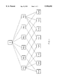
FIG. 1 is an illustration useful in understanding the operation of the invention and represents all of the possible populations associated with an illustrative data set.
FIG. 2 is a flowchart describing the process of the preferred embodiment.
OPERATION
Using the novel method of the invention (called attribute inductive data analysis or "AIDA") data sets are analyzed to identify sources of variations in a response variable associated with the data. To illustrate how AIDA identifies sources of variations, an illustrative data set will be considered. Table 1 lists defect data that might be derived from an illustrative manufacturing process in which four machines (M1, M2, M3 and M4) were used to produce two types of products, namely, product one (P1) and product two (P2).
              TABLE 1
______________________________________
P.sub.1            P.sub.2 Total
______________________________________
M.sub.1 1/25           2/75    3/100
M.sub.2 3/25           3/75    6/100
M.sub.3 4/25           11/75   15/100
M.sub.4 1/25           1/75    2/100
Total    9/100         17/300
______________________________________
The numerators in each fraction represent the number of defects while the denominators represent the total number of products produced. For example, each machine produced twenty-five products P1 and seventy-five products P2 and machine M3 produced four defective products P1 and eleven defective products P2.
The AIDA method, as applied to this data set, may be used to identify possible sources of variations in the response variable (which in this case is the fraction defective). In other words, if the manufacturing process has a source of defects, it will be manifested by a variance in the fraction defective among populations in the data set, as explained more fully below. For example, if machine M1 is not properly set up to produce products P2, this may result in a higher incidence of defects for products P2 that are produced on machine M1 while products P2 produced by the other machines and other products produced by machine M1 should not be responsible for sources of variations.
The invention comprises a system that first organizes the data into populations, each population determined by either a single attribute or a conjunction of zero or more attributes (a universe population is defined as being specified by the union of all other populations, and therefore specifies the entire data set). In the illustrative manufacturing process the attribute values are M1, M2, M3, M4, P1 and P2. FIG. 1 shows all of the possible populations derived from the illustrative data set. The universe population ("U") appears at the top of the figure with populations defined by single attributes shown as "subpopulations" of U. For example, the population M1p is defined as data derived from products produced by M1. The subpopulations of each of the single attribute populations are then shown in the bottom of FIG. 1. For example, the population specified by the conjunction of P1p and M3p (i.e.,P1p M3p) is both a subpopulation of P1p and a subpopulation of M3p and represents the products P1 produced by M3 (i.e. the intersection of P1p and M3p). Populations P1p and M3p are also referred to as "parent" populations of P1p M3p. It should be readily apparent that in a complicated manufacturing process with many attributes, the total number of populations would be enormous and the set relations extrememly complex.
The system begins its search for sources of variation by defining a test population as being the universe population (see step 1 in FIG. 2). Next, each subpopulation of the test population is evaluated to determine: (1) which of the subpopulations has the most significant variation; and (2) whether the chosen subpopulation is a "significant" population (step 2 in FIG. 2). To determine the significance of a population's variation, it is compared with its complement. The complement of a population is that portion of the data set that remains when the population is subtracted from or removed from the data set. The complement of a subpopulation with respect to a parent population is all the data in the parent which remains when the subpopulation is subtracted from the parent.
The comparison of a population to its complement (i.e. step 2) is performed by calculating its "Z-Complement." The Z-Complement is a known statistical approximation for the comparison of probabilities of two binomial distributions. See, e.g., Lothar Sachs, Applied Statistics, page 338 (1982). In the context of this example, the Z-Complement is defined as a numerical measurement for the probability that a specific population has an intrinsically higher fraction defective than its complement. In other words, since the data set being analyzed is only representative of the manufacturing process, it is not an exact measurement of the true defect rate inherent in the process. However, the larger a variation in the fraction defective the higher the probability the variation is intrinsically greater than that for its complement. The Z-Complement measures this probability and is measured in units of standard deviations. As an example, a Z-Complement of 1.0 corresponds to a probability of 84.1%, while a Z-Complement of 3.0 corresponds to a probability of 99.9%.
To calculate the Z-Complement of M1p, the fraction defective of M1p ("F") is first calculated as follows: ##EQU1## where X equals the total number of defects in the population and N equals the total number of opportunities for defects for the population of interest. For example, the number of opportunities for defects for the population M1p is the total number of products associated with this population (i.e., the total number of products produced by M1). Referring to Table 1 above, it can be seen that for M1, X=3 and N=100. Therefore, for M1p F equals 0.030. The fraction defective of the complement of M1p with respect to the current test population (the complement consisting of M2p +M3p +M4p) is then calculated as follows: ##EQU2## where F' is the complement fraction defective, X' is the total number of defects for the complement and N' is the total number of opportunities for defects. Referring again to Table 1, X' equals the total number of defects for M2p, M3p and M4p combined (i.e., M1p 's complement) which is 23. The total number of opportunities, N', is 300. Therefore F' equals 0.076. The Z-Complement ("Z") M1p can now be calculated as follows: ##EQU3## where Fp, the pooled fraction defective, is defined by the following: ##EQU4##
Performing these calculations for the data associated with M1p results in a Z-complement value of -1.64. Table 2 lists the calculated values for each subpopulation of the current test population (the universe population).
              TABLE 2
______________________________________
Subpopulation Data
                 Complement Data
Frac. Def.   F       Frac. Def.  F'   Z
______________________________________
M.sub.1p
       3/100     .030    23/300    .077 -1.64
M.sub.2p
       6/100     .060    20/300    .067 -0.23
M.sub.3p
       15/100    .150    11/300    .037 3.98
M.sub.4p
       2/100     .020    24/300    .080 -2.11
P.sub.1p
       9/100     .090    17/300    .057 1.17
P.sub.2p
       17/300    .056     9/100    .090 -1.17
______________________________________
The system then compares the highest subpopulation Z-Complement to a threshold value to determine if it is a significant population (step 3 in FIG. 2). The threshold value is selected considering the acceptable level of risk that an identified population may not have an intrinsically higher fraction defective and is therefore not a true source of varience. If the threshold in this example is set at 4.00, then M3p, which has the highest Z-Complement, will not be a significant population, and there will be no significant subpopulations for this test population. Since the current test population is the universe population, the process will be finished (step 5 in FIG. 2), and the conclusion will be that there are no significant sources of variation for this data set. In other words, the defects are distributed throughout the data set such that it cannot be stated, with the degree of certainty determined by the threshold (which approaches a probability of 100% since the threshold is 4.0), that any one population is responsible for an unusually high number of defects.
However, it will be assumed that the threshold is, e.g. 3.0 (corresponding to a 99.9% probability), so M3p will be deemed a significant population (step 3) and will become the new test population (step 4).
The system then continues and examines the subpopulations of the new test population (step 2). Referring to FIG. 2, it can be seen that the subpopulations of M3p are P1p M3p and P2p M3p. Performing the same mathematical calulations described above for these subpopulations results in the data in Table 3. Note that the complements are always defined with respect to the current test population. For example the complement of P1p M3p with respect to M3p is P2p M3p whereas the complement of P1p M3p with respect to P1p is the combination of P1p M1p, P1p M2p and P1p M4p. Accordingly, since the current test population is M3p, the proper complement of P1p M3p is P2p M3p and the complement of P2p M3p is P1p M3p.
              TABLE 3
______________________________________
Subpopulation Data
                  Complement Data
Frac. Def.   F        Frac. Def. F'   Z
______________________________________
P.sub.1p M.sub.3p
         4/20    .200     11/80    0.137
                                        .70
P.sub.2p M.sub.3p
        11/80    .137      4/20    0.200
                                        -.70
______________________________________
While P1p M3p has a higher Z-Complement than P2p M3p, its Z-Complement is not greater than the threshold (step 3). Since the current test population (i.e., M3p) is not the universe population (step 5), the system will add M3p as the new "cover" (the use of the term cover is explained below).
The data is revised as if the defects produced by M3 never occurred (step 6). The populations affected will be M3p and any intersecting populations (i.e. P1p, P2p, P1p M3p and P2p M3p). Once the system locates a source of variance in the data set, it revises the data to eliminate that source (i.e., the defect data is "covered"). The revised data set can now be evaluated to determine if other sources of variance in the fraction defective exist which are independent of the source associated with the covered population (i.e., independent of M3p). Since the cover is an isolated source of variation, it is added to a list of isolated sources of variation as is each cover determined throughout the process (step 7). The revised data set appears in Table 4.
              TABLE 4
______________________________________
P.sub.1            P.sub.2 Total
______________________________________
M.sub.1 1/25           2/75    3/100
M.sub.2 3/25           3/75    6/100
M.sub.3 0/25           0/75    0/100
M.sub.4 1/25           1/75    2/100
Total    5/100          6/300
______________________________________
To locate these other possible sources, the system returns to step 1 in FIG. 1 and again sets the test population equal to the universe population (note that the universe population is now defined with respect to the revised data set). All of the Z-Complements are calculated based on the revised data set using the formulas described above. Table 5 lists the results of these calculations.
              TABLE 5
______________________________________
Subpopulation Data
                  Complement Data
Frac. Def.    P       Frac. Def. P'   Z
______________________________________
M.sub.1p
       3/100      .030    8/300    .027 0.18
M.sub.2p
       6/100      .060    5/300    .017 2.29
M.sub.3p
       0/100      .000    11/300   .037 -1.94
M.sub.4p
       2/100      .020    9/300    .030 -0.53
P.sub.1p
       5/100      .050    6/300    .020 1.59
P.sub.2p
       6/300      .020    5/100    .050 -1.59
______________________________________
The revisions to the data set caused by covering M3p are apparent in Table 5. While the individual fraction defectives of the other machine populations remain the same, the complement data is affected and the resulting Z-Complement values are changed.
Using the same threshold as above (i.e., 3.0), the system would conclude that M2p, the subpopulation with the highest fraction defective, is not a significant subpopulation (step 3) and, since our test population is the universe population, the process would end (step 5).
It should now be apparent that the lower the threshold the more sensitive the analysis becomes. A very low threshold will generally result in more sources of variation being isolated.
To summarize the AIDA system, the universe population is initially chosen as a test population and each of its subpopulations is evaluated to see if one is significantly different from the others. If none are, then the defects are fairly evenly dispersed throughout the data set and there is no one particular source of variance in terms of the attributes being evaluated. If, however, one of the subpopulations is significant then the system makes that subpopulation the new test population to see if the source of variance can be narrowed down even further. Accordingly, referring to FIG. 1, the system starts at the top of the figure and proceeds down from one population to another to locate sources of variance. When it locates such a source, it "covers" it and starts over again to look for other sources of variation. This process continues until no new sources of variation can be located.
When the process has been completed, the resulting information (the individual covers) can be used to help infer root causes regarding defects in the manufacturing process itself. For example, M3p was determined to be the only source of variation in the above example (using a threshold of 3.0) which might indicate that M3 is not operating properly. Since the other three machines produce the same products as this machine, we may infer that the products themselves are not defective, (e.g., due to bad raw materials) but that the fault lies with M3.
Although a relatively simple data set was analyzed above, other data sets can have many attributes. Furthermore, the illustrative data set was uniform (e.g. each machine produced 100 products), but the system can be used to analyze non uniform data sets, even if some populations are empty.
Other embodiments of the invention are within the scope of the appended claims.